Equations for a function

Almost every quantitative law in science says something about a rate of change rather than about a value, so the thing it pins down is a function and not a number.

Ernest Rutherford and Frederick Soddy found in 1902 that a radioactive sample loses atoms at a rate proportional to how many it still has. That sentence is not a formula for the number of atoms. It is a constraint linking the unknown function $N (t)$ to its own derivative, $\frac{d N}{d t} = - k N$ , and the work of extracting $N (t)$ from it is what this course is about. Newton's second law is the same kind of statement, one derivative further along: force is mass times acceleration, and acceleration is the second derivative of position, so every mechanical problem arrives as a constraint on $x (t)$ and $x'' (t)$ rather than as a recipe for $x$ .

This lesson assumes the derivative rules and definite integration from the previous course, and nothing else. It sets up the vocabulary, then shows the one thing that can always be done to a differential equation even when it cannot be solved.

A law of change is an equation for a curve

A differential equation is an equation relating an unknown function to one or more of its derivatives. A solution is a function that satisfies it on some interval, and the word "some" is doing real work there, as the end of the lesson shows.

The distinction from ordinary algebra is worth making slowly, because it is where beginners lose their footing. Solving $x^{2} - 5 x + 6 = 0$ produces two numbers, $2$ and $3$ , and checking them is arithmetic. Solving $y' = 2 y$ produces a family of functions, $y = C e^{2 t}$ for every constant $C$ , and checking one is differentiation. The unknown lives in a space of functions, so the answer is a curve, or rather infinitely many curves, one through every point of the plane.

We restrict to ordinary differential equations, where the unknown depends on one variable, almost always time. If the unknown depends on several variables, the derivatives are partial and the equation is a partial differential equation: the heat equation and the wave equation are the standard examples, and they need machinery beyond this course. Everything here is one independent variable, which is enough for mechanics, circuits, chemical kinetics and population models.

Order, linearity, and why the labels stick

Two labels decide which method will work, so they are worth fixing before any method exists.

The order is the highest derivative that appears. $\frac{d N}{d t} = - k N$ is first order. The spring equation $m x'' + c x' + k x = 0$ is second order. Order is not a matter of taste: it counts how much information you must supply to select one solution out of the family, and it is why a projectile needs both a launch position and a launch velocity while a decaying sample needs only its starting mass.

An equation is linear if the unknown and its derivatives appear only to the first power, never multiplied together, and never inside a function like $\sin$ or a square root. The general linear equation of second order is

a_{2} (t) y'' + a_{1} (t) y' + a_{0} (t) y = g (t)

where the coefficients may be any functions of $t$ at all. Linearity is a statement about how $y$ enters, not about how $t$ enters: $y' + t^{2} y = \cos t$ is linear, and $y' = y^{2}$ is not. If $g (t)$ is zero the linear equation is called homogeneous, and if not, the term $g$ is the forcing.

Linear equations are the ones with a complete theory, because solutions can be added: if $y_{1}$ and $y_{2}$ both solve a homogeneous linear equation, so does $y_{1} + y_{2}$ . Try that on $y' = y^{2}$ . With $y_{1} = - 1 / t$ and $y_{2} = - 1 / (t + 1)$ , both genuine solutions, the sum satisfies nothing at all. Nonlinear equations lose superposition, and with it most of the algebra, which is why the second half of this course spends its effort on reading nonlinear solutions rather than writing them.

Verifying a solution

Checking a candidate needs no theory: differentiate it, substitute, and see whether the two sides agree for every $t$ in the interval, not just at one point.

Example. Show that $y = 3 e^{2 t} - 2 e^{- t}$ solves $y'' - y' - 2 y = 0$ , and find $y (0)$ and $y' (0)$ .

Differentiating, $y' = 6 e^{2 t} + 2 e^{- t}$ and $y'' = 12 e^{2 t} - 2 e^{- t}$ . Substituting,

(12 e^{2 t} - 2 e^{- t}) - (6 e^{2 t} + 2 e^{- t}) - 2 (3 e^{2 t} - 2 e^{- t})

The $e^{2 t}$ terms give $12 - 6 - 6 = 0$ and the $e^{- t}$ terms give $- 2 - 2 + 4 = 0$ , so the left side is identically zero and the candidate is a solution. At $t = 0$ , $y (0) = 3 - 2 = 1$ and $y' (0) = 6 + 2 = 8$ .

Now you. Show that $y = C_{1} e^{3 t} + C_{2} e^{- 2 t}$ solves $y'' - y' - 6 y = 0$ for every pair of constants, and find $y (0)$ and $y' (0)$ in terms of $C_{1}$ and $C_{2}$ .

Answer

$y' = 3 C_{1} e^{3 t} - 2 C_{2} e^{- 2 t}$ and $y'' = 9 C_{1} e^{3 t} + 4 C_{2} e^{- 2 t}$ . The $e^{3 t}$ coefficient is $9 - 3 - 6 = 0$ and the $e^{- 2 t}$ coefficient is $4 + 2 - 6 = 0$ , so the equation holds for any $C_{1}$ and $C_{2}$ . At $t = 0$ , $y (0) = C_{1} + C_{2}$ and $y' (0) = 3 C_{1} - 2 C_{2}$ .

Verification is cheap and solving is expensive, which is a lopsidedness worth exploiting. Guessing a form, substituting it, and letting the equation fix the constants is a legitimate and heavily used method, and it is exactly how the constant-coefficient theory later in this course is built.

Why solutions come in families

The simplest differential equation is $y' = f (t)$ , whose solution is an antiderivative of $f$ . There is never exactly one: antiderivatives differ by a constant, so the answer is a family $y = F (t) + C$ , and that single arbitrary constant is the residue of everything the equation does not know. The equation constrains the slope at every instant and says nothing about where the curve starts.

That generalises. An equation of order $n$ has a general solution carrying $n$ arbitrary constants, and a particular solution is one member of the family with the constants fixed. The count matches the order because integrating $n$ times introduces $n$ constants, and it is the reason order is the first thing to identify.

To select a member you supply extra data. An initial value problem gives the value of the function and of its first $n - 1$ derivatives at one instant $t_{0}$ . For a second order equation that is a position and a velocity, which is precisely the state Newtonian mechanics says determines a trajectory. Supplying data at two different instants instead, such as $y (0) = 0$ and $y (1) = 0$ , makes it a boundary value problem, which behaves quite differently: such problems can have no solution or infinitely many, and this course stays with initial conditions.

Example. The general solution of $y'' + 4 y = 0$ is $y = A \cos 2 t + B \sin 2 t$ , which you can check by substituting. Solve the initial value problem with $y (0) = 3$ and $y' (0) = 8$ , and give the amplitude of the resulting oscillation.

Setting $t = 0$ in $y$ gives $y (0) = A = 3$ . Differentiating, $y' = - 2 A \sin 2 t + 2 B \cos 2 t$ , so $y' (0) = 2 B = 8$ and $B = 4$ . The particular solution is $y = 3 \cos 2 t + 4 \sin 2 t$ . Combining the two terms into a single sinusoid gives amplitude $\sqrt{A^{2} + B^{2}} = \sqrt{9 + 16} = 5$ , so the motion runs between $- 5$ and $5$ .

Now you. For the same equation, solve the initial value problem with $y (0) = - 2$ and $y' (0) = 12$ , and give the amplitude.

Answer

$A = - 2$ , and $y' (0) = 2 B = 12$ gives $B = 6$ . So $y = - 2 \cos 2 t + 6 \sin 2 t$ , with amplitude $\sqrt{4 + 36} = \sqrt{40} = 6.32$ .

Building the equation from the words

Most of the difficulty in applying this subject is not solving the equation but writing it down, and writing it down is always the same move: express the rate of change of the quantity as the sum of everything adding to it minus everything removing it.

Take the decay law. In one year a radiocarbon sample loses a fixed fraction of whatever it has, so $\frac{d N}{d t} = - k N$ , and the constant is fixed by the measured half-life of $5730$ years for carbon-14. Setting $N = N_{0} / 2$ in the solution $N = N_{0} e^{- k t}$ gives $k = \ln 2 / 5730 = 1.210 \times 10^{- 4}$ per year. That number then dates anything organic: a sample holding $78$ per cent of its original carbon-14 has been dead for $\ln (1 / 0.78) / k = 2054$ years.

Take a falling body with air resistance. Gravity pulls down with force $m g$ , drag opposes motion with a force that at everyday speeds is close to proportional to $v^{2}$ , and Newton's law assembles them into

m \frac{d v}{d t} = m g - b v^{2}

first order, nonlinear because of the square, and already interesting before it is solved: whenever $b v^{2}$ reaches $m g$ the derivative vanishes and the speed stops changing. That terminal speed is $\sqrt{m g / b}$ , read off the equation itself without any solving. A skydiver in a spread posture has $m / b$ near $300$ m, giving $\sqrt{300 \times 9.81} = 54$ m s⁻¹, or about $195$ km h⁻¹, which is the figure the sport quotes.

Take a mixing tank. Brine at $c_{in}$ kilograms per cubic metre enters at $q$ cubic metres per minute, the tank holds $V$ cubic metres and is stirred so its concentration is uniform, and the outflow matches the inflow. The salt mass $S$ changes at the rate it enters minus the rate it leaves, $\frac{d S}{d t} = q c_{in} - \frac{q}{V} S$ : first order and linear, and the model for every stirred reservoir from a chemical reactor to a lake.

Direction fields: the family without the formula

Here is the move that makes an unsolvable equation useful. A first order equation $y' = f (t, y)$ hands you the slope of the solution at every point of the plane before you know any solution. Draw a short segment of that slope at each of a grid of points and you have a direction field: solutions are exactly the curves that stay tangent to it everywhere, and the eye assembles them from the picture.

Consider $y' = t - y$ . At the point $t = 1$ , $y = 2$ the slope is $1 - 2 = - 1$ . On the line $y = t$ every slope is zero, so solutions crossing that line do so horizontally. Above it slopes are negative and below it positive, so every solution is pushed towards the line from both sides. The line itself is nearly a solution: trying $y = t - 1$ gives $y' = 1$ and $t - y = 1$ , so it is a solution exactly. The picture says that whatever a solution does early on, it ends up hugging $y = t - 1$ , and this is right: the general solution turns out to be $y = t - 1 + C e^{- t}$ , and the $C e^{- t}$ term dies.

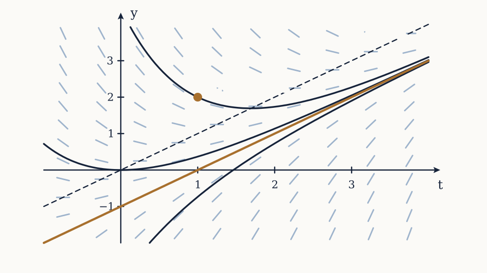
A curve on which the slope takes one fixed value is an isocline, and sketching a few is the fast way to draw a field by hand. For $y' = t - y$ the isoclines are the straight lines $t - y = m$ , one per slope $m$ .

Example. For $y' = y (1 - y)$ , find the slope at $y = 0.5$ , at $y = 2$ and at $y = 1$ , and say what a solution starting at $y (0) = 0.5$ does.

The slopes are $0.5 \times 0.5 = 0.25$ , then $2 \times (1 - 2) = - 2$ , then exactly $0$ . Since $f$ does not involve $t$ , the slope depends only on the height, so each horizontal line carries a single slope. The lines $y = 0$ and $y = 1$ carry slope zero and are constant solutions. Between them the slope is positive, so a solution starting at $0.5$ rises, and since it can never cross the constant solution at $y = 1$ , it approaches $1$ from below without reaching it. Above $y = 1$ slopes are negative, so those solutions fall to $1$ as well.

Now you. For $y' = 2 - y$ , give the slope at $y = 0$ , $y = 2$ and $y = 5$ , and say what happens to a solution starting at $y (0) = 5$ .

Answer

The slopes are $2$ , $0$ and $- 3$ . The constant solution is $y = 2$ , and a solution starting at $5$ has negative slope, so it falls, slowing as it goes, and approaches $2$ from above without crossing it.

What is actually solvable

An honest course says early what its methods will not reach. Almost every differential equation you can write down has no solution expressible in elementary functions. $y' = t^{2} + y^{2}$ is about as simple as an equation gets, and its solutions require Bessel functions; $y' = e^{- t^{2}} + y$ pulls in the error function immediately. This is not a gap in the textbooks. It is the same fact as most integrals having no elementary antiderivative, since integration is the special case $y' = f (t)$ .

So the subject has three tools rather than one, and they will be used throughout. Exact solution, where a formula exists and is worth having. Qualitative analysis, which reads the long-term behaviour off the equation itself, as the terminal speed and the direction field did above. Numerical solution, which produces a table of values to whatever accuracy is paid for. A good answer often uses all three: the numerics give the curve, the qualitative argument says the curve is believable, and the exact solution of a simplified version says what controls it.

Solutions also have limited lifetimes. $y' = y^{2}$ with $y (0) = 1$ has the solution $y = 1 / (1 - t)$ , which is perfectly well behaved near $t = 0$ and infinite at $t = 1$ , even though the equation itself shows no sign of trouble there. A differential equation is a local statement, and asking where its solutions stop existing is a real question, taken up in a later lesson.

The next step is the first class of equations that yields completely. When the right side factors into a function of $t$ times a function of $y$ , the variables can be separated and both sides integrated, which turns the decay law, the cooling law and the logistic curve into three lines of calculus each.