Microeconomics

Economics is not the study of money, and a course that begins with money will be lost by the third lesson.

Lionel Robbins gave the definition that still works, in his Essay on the Nature and Significance of Economic Science of 1932: economics is the science which studies human behaviour as a relationship between ends and scarce means which have alternative uses. Every word of that is load-bearing. There are ends, plural, so ranking is required. The means are scarce, so not all ends can be met. And the means have alternative uses, so committing them to one end withdraws them from another. Strip out the money and the markets and what is left is a maximisation subject to a constraint, which is a problem in calculus. This course is that problem, solved over and over with different objects in it.

Scarcity is a constraint, not a shortage

A shortage is a temporary failure to supply something: no eggs on the shelf this morning. Scarcity is permanent and applies to things that are abundant. There is a great deal of drinking water on Earth, and water is scarce in the economic sense, because using a litre to cool a data centre is using a litre that cannot irrigate a field. Scarcity means only that the resource has more claims on it than it can meet at once.

So the honest form of any economic question is not "is this worth doing" but "is this worth doing with resources that could do something else". Time is the cleanest example because nobody can accumulate it: a day is 24 hours for a billionaire and for a bankrupt, and every hour spent is an hour withheld from every other use. Diamonds are expensive and time is priceless, but only one of them is genuinely fixed in supply.

The subject splits into two kinds of claim, and mixing them is the most common way to argue past someone. A positive claim says what is: a tax of this size will cut consumption by that much. It can be wrong, and evidence settles it. A normative claim says what ought to be: that cut is worth its cost. It cannot be settled by evidence alone, because it rests on how the losses to some are weighed against the gains to others. Most of this course is positive. The welfare lessons later on are where the boundary has to be watched hardest, and the honest position there is that the model can say what is efficient and cannot, by itself, say what is good.

Opportunity cost

If the means have alternative uses, then the cost of using them one way is the best alternative given up. That is the opportunity cost, and it is the only cost that belongs in a decision. Money paid out matters only when it stands for something forgone; money not paid out matters just as much when something was forgone anyway.

Two consequences follow immediately, and both catch people. First, a cost you would bear whichever way you choose is not a cost of the choice. Second, a resource you already own is not free to use, because it could have been sold or rented to someone else.

Example. A student is deciding whether to take a three-year degree in England, where the tuition fee cap for a home undergraduate was £9,250 a year from 2017 to 2024. The alternative is a job paying £20,000 a year. Rent and food come to £9,000 a year and would be paid either way. What is the opportunity cost of the degree?

The fees are £9,250 × 3 = £27,750, and they are paid only in the degree branch, so they count. The forgone wages are £20,000 × 3 = £60,000, and they count too, even though no cheque is written for them, because they are the best alternative use of the same three years. Rent and food do not count at all: £27,000 over three years appears in both branches and cancels. So the opportunity cost is £27,750 + £60,000 = £87,750, of which more than two thirds is money nobody ever sees on an invoice. This is why the fee debate and the cost of a degree are different subjects.

Now you. The same student instead considers a two-year apprenticeship with no fees, paying £12,000 a year, against the same £20,000 job. What is the opportunity cost of the apprenticeship?

Economists are not reliably better at this than anyone else. Paul Ferraro and Laura Taylor put a four-option opportunity cost question to professional economists at the 2005 American Economic Association meetings, about the value of a free concert ticket, and 21.6 per cent chose the right answer. Random guessing would have scored 25. The concept is easy to state and genuinely hard to apply, which is why it is worth practising rather than merely reading.

The production possibility frontier

Put the idea on a diagram. Take an economy with one resource, 100 hours of labour a day, and two goods, fish and coconuts. Suppose catching $F$ fish takes $F^2/100$ hours and gathering $C$ coconuts takes $C^2/25$ hours. Both are convex in output, which is the assumption that the easy fish are caught first and each additional one is harder. Using all the labour,

or, cleared of fractions, $F^2+4C^2=10000$. That curve is the production possibility frontier: every combination on it uses the whole resource, everything inside it is feasible but wasteful, and everything outside it is impossible with today's technology. Setting $C=0$ gives 100 fish, and setting $F=0$ gives 50 coconuts.

Three readings of the picture matter. A point strictly inside the curve means unemployment or misallocation, and moving to the frontier gives more of both goods with no sacrifice, which is why the phrase "no such thing as a free lunch" is a statement about points on the frontier only. A point outside is reachable only by acquiring more resources or better technology, which is what growth is. And on the frontier itself, more of one good is available only at the price of less of the other, which is opportunity cost drawn as a slope.

The slope is a price

Differentiate the frontier implicitly, which is what implicit differentiation is for: $2F\mathrm{d}F+8C\mathrm{d}C=0$, so

The magnitude of that slope is the marginal rate of transformation: how many coconuts one more fish costs at the margin. It is not a fixed number. At $F=60$ the constraint gives $4C^2=10000-3600=6400$, so $C=40$, and the rate is $60/160=0.375$ coconuts per fish. Push production to $F=80$ and $C$ falls to 30, and the rate rises to $80/120=0.67$ coconuts per fish. The more fish already being caught, the more each extra fish costs, which is exactly the curvature the assumption about hard fish put in.

Example. On the same frontier $F^2+4C^2=10000$, the economy is at $F=60$. It wants ten more fish. Estimate the coconut cost using the marginal rate, then compute it exactly, and say why the two differ.

The marginal rate at $F=60$ is 0.375, so ten fish look like a sacrifice of 3.75 coconuts. Exactly: at $F=70$, $4C^2=10000-4900=5100$, so $C=35.71$, a fall of 4.29 coconuts. The linear estimate understates the cost because the rate is rising over the interval, and it is evaluated only at the start. Marginal reasoning is a first derivative, so it is exact for a small step and an approximation for a large one, a caveat worth carrying through the whole course.

Now you. On the same frontier, find the marginal rate of transformation at $F=80$, and the exact coconut cost of moving from $F=80$ to $F=90$.

The same slope reasoning is what settles who should produce what. If a second island gives up only 0.2 coconuts per fish where this one gives up 0.375, the second island has the lower opportunity cost in fish, and both gain from specialising and trading at any rate between the two. That is comparative advantage, and it depends on the ratio of the slopes, never on who is better at things in absolute terms.

Thinking at the margin

Now the rule the rest of the course runs on. Suppose an activity produces benefit $B(x)$ and costs $C(x)$, both differentiable. The net gain is $B(x)-C(x)$, and at an interior maximum its derivative vanishes:

Do the thing until the marginal benefit of one more unit equals the marginal cost of it. This is not a new economic principle. It is the first-order condition from calculus, with the two derivatives given names, and it is worth saying so plainly, because it means the economics is entirely in the choice of $B$ and $C$ and never in the mathematics.

Two conditions have to hold for the rule to be right, and both fail in real problems often enough to be worth stating. The stationary point must be a maximum rather than a minimum, so $B^{\prime \prime }<C^{\prime \prime }$ there, which is the usual second derivative test and is the formal content of "diminishing returns". And the optimum must be interior. If marginal benefit is below marginal cost at every positive $x$, the answer is $x=0$ and the derivatives never meet: the right amount of a bad investment is none of it, and no first-order condition will tell you that. Corner solutions come back properly in the consumer's problem two lessons from now.

The rule also explains why totals mislead. Water is worth more to a human being than diamonds are, and yet diamonds trade for more. Adam Smith found this genuinely puzzling in 1776. The resolution is that no one ever chooses between all the water and all the diamonds. The choice on offer is one more litre against one more carat, and where water is abundant the marginal litre is worth almost nothing while the marginal carat is not. Price tracks marginal value, not total value, and almost every paradox about what things are worth dissolves into that distinction.

Equalising at the margin

When one fixed resource is split between several uses, the marginal rule becomes an equalisation. If it were true that the last pound spent in one place bought more than the last pound spent in another, moving a pound would raise the total, so no such gap can survive at the optimum.

Example. A firm has £26,000 to spend on advertising in two regions. Revenue in region A is $60\sqrt{a}$ thousand pounds when $a$ thousand is spent there, and revenue in region B is $40\sqrt{b}$. How should the budget be split?

The marginal returns are $\mathrm{d}{R}_A/\mathrm{d}a=30/\sqrt{a}$ and $\mathrm{d}{R}_B/\mathrm{d}b=20/\sqrt{b}$. Setting them equal gives $30/\sqrt{a}=20/\sqrt{b}$, so $\sqrt{a}=1.5\sqrt{b}$ and $a=2.25b$. With $a+b=26$ that gives $3.25b=26$, so $b=8$ and $a=18$. Both marginal returns are then $30/\sqrt{18}=20/\sqrt{8}=7.07$ thousand pounds per thousand spent. Total revenue is $60\sqrt{18}+40\sqrt{8}=367.7$ thousand, against 360.6 thousand for an even split of 13 and 13. The even split feels fair and costs £7,100.

Now you. The budget is £40,000, region A still returns $60\sqrt{a}$, and region B now returns only $30\sqrt{b}$. Find the split and the total revenue.

What is not a cost

The mirror image of opportunity cost is the sunk cost: money or effort already committed and unrecoverable whatever happens next. It appears in no branch of the decision, so it cancels exactly as the rent did, and the correct treatment is to ignore it entirely.

People do not. Hal Arkes and Catherine Blumer ran the clean demonstration in 1985, selling season tickets to the Ohio University theatre and randomly discounting some buyers to two thirds or roughly half the normal price without telling them the discount was coming. All three groups had identical tickets and identical plays ahead of them, and the only difference was money already spent. Full-price buyers attended significantly more plays in the first half of the season. The past payment changed behaviour that it could not rationally affect. The pattern has a name in policy too: the British and French governments continued funding Concorde long after the projected returns had collapsed, on the argument that too much had already been spent to stop.

This is the first place where the model and the people come apart, and it will not be the last. The claim that people ignore sunk costs is false as a description and useful as a prescription, and those are different claims about the same sentence. Keeping them separate is most of what it takes to use this subject honestly. The final lesson returns to the evidence in full.

What the rule still lacks is a measure of benefit. Every optimisation so far has assumed a function $B(x)$ handed over from outside: revenue in pounds, coconuts on a frontier. For a consumer choosing between goods there is no such natural unit, only the fact that they prefer some bundles to others. Turning a ranking into a differentiable function is the next lesson's problem, and it turns out to need surprisingly little.

The marginal rule from the previous lesson needs a benefit function, and for a person choosing between goods there is no obvious unit to measure benefit in.

Jeremy Bentham thought there was. His felicific calculus of 1789 treated pleasure as a quantity with an intensity and a duration, addable across people, and for a century economists wrote as though a unit of satisfaction were a physical measurement waiting for a better instrument. It is not. Nobody has ever measured a util, and no experiment could, because there is nothing there to measure. What can be observed is choice: offered two bundles of goods, a person takes one. Everything in this lesson is built out of that observation and nothing else, which turns out to be enough.

The ranking is the primitive

Start with a consumption bundle, a list of quantities of each good. With two goods it is a point $(x,y)$ in the positive quadrant, and the two-good case is not a simplification so much as a drawing convention: let $y$ stand for "money spent on everything else" and any problem becomes two-dimensional.

The primitive object is a relation on bundles. Write $A⪰B$ for "the consumer finds $A$ at least as good as $B$". From it, two others are defined rather than assumed: $A$ is strictly preferred to $B$ when $A⪰B$ holds and $B⪰A$ does not, and $A$ is indifferent to $B$ when both hold. Notice what has not been said. There is no number attached to $A$, no claim about how much better it is, and no comparison with anyone else's ranking. A ranking is all the data there is.

Four assumptions, and what each buys

An arbitrary relation is useless, so preferences are restricted. Four assumptions do the work, and it is worth knowing which result each one is paying for, because they are not equally innocent.

Completeness. For any two bundles, at least one of $A⪰B$ and $B⪰A$ holds. The consumer is never unable to say. This rules out "I have no idea", which is a real state of mind, and it is the assumption that makes the whole quadrant rankable rather than partly rankable.

Transitivity. If $A⪰B$ and $B⪰C$ then $A⪰C$. Without it there is no best element to find: a consumer preferring $A$ to $B$, $B$ to $C$ and $C$ to $A$ can be walked around the cycle for a small fee at each step and returned to where they started, poorer, forever. Transitivity is what makes maximisation meaningful at all.

Monotonicity, or non-satiation. More of a good is better. This is what makes them goods, and it fixes the direction of every diagram: north-east is up.

Continuity. If a sequence of bundles all at least as good as $B$ converges to some bundle $A$, then $A$ is at least as good as $B$ too. Preferences have no sudden jumps. This is the technical assumption, the one with no intuitive content, and it is the one that earns the representation theorem.

Gerard Debreu proved in 1954 that complete, transitive, continuous preferences over a connected set of bundles can be represented by a continuous utility function: a function $u$ with $u(A)\ge u(B)$ exactly when $A⪰B$. That theorem is the licence for everything that follows. It says a numerical function exists, so calculus applies, and it says nothing whatever about the function being unique or meaningful.

Indifference curves

Fix a value $\bar{u}$ and look at the set of bundles satisfying $u(x,y)=\bar{u}$. That level set is an indifference curve, and the family of them is a contour map of the preference ranking. Francis Edgeworth drew the first ones in Mathematical Psychics in 1881, and Vilfredo Pareto in 1906 made the decisive point that the contours carry all the information and the labels on them do not.

Three properties follow from the assumptions rather than from drawing habit. Indifference curves slope downward, because monotonicity says that giving up some $x$ must be compensated with more $y$ to stay level. Curves further from the origin are better, for the same reason. And two indifference curves cannot cross: if they did, the crossing point would be indifferent to a bundle on each curve, and transitivity would force those two bundles to be indifferent to each other, contradicting the fact that one lies north-east of the other.

Utility represents, it does not measure

Here is the point that separates modern consumer theory from Bentham. If $u$ represents a preference ranking and $f$ is any strictly increasing function, then $f(u)$ represents exactly the same ranking, because applying an increasing function to both sides of an inequality leaves the inequality alone. Utility is ordinal: only the order of the numbers means anything. Their size, their differences, and their ratios do not.

Example. Take $u(x,y)=\sqrt{xy}$, and compare the bundles $A=(4,9)$ and $B=(8,4)$. Now repeat with $v=xy$ and with $w=\ln x+\ln y$, and check that the ranking survives.

Under $u$: $u(A)=\sqrt{36}=6$ and $u(B)=\sqrt{32}=5.66$, so $A$ wins. Under $v$: $v(A)=36$ and $v(B)=32$, so $A$ wins. Under $w$: $w(A)=\ln 36=3.584$ and $w(B)=\ln 32=3.466$, so $A$ wins. All three are increasing transformations of one another, since $v=u^2$ and $w=\ln v$, so no ranking could have differed. But note what did change: under $u$ the gap is 0.34, under $v$ it is 4, and under $w$ it is 0.118. Any statement of the form "$A$ is six per cent better" is a statement about the arbitrary labelling and not about the consumer.

Now you. Using the same three functions, rank $A=(4,9)$ against $C=(6,6)$, and say what the answer means.

The practical consequence is a rule for later lessons. Any result that changes when utility is relabelled is an artefact and must be thrown away. Interpersonal comparisons are the biggest casualty: since each person's utility number is arbitrary up to an increasing transformation, adding two people's utilities together is arithmetic on units that do not exist. That does not make the comparison meaningless as a moral matter, but it does mean the model cannot supply it, and the welfare lessons will have to work with something weaker.

The marginal rate of substitution

Something must survive relabelling, or the theory would say nothing. What survives is the slope of the indifference curve.

Marginal utility is a partial derivative, ${\mathrm{MU}}_x=\partial u/\partial x$, the rate at which utility rises with $x$ holding $y$ fixed. On its own it is as arbitrary as utility itself: replace $u$ by $u^2$ and every marginal utility doubles at $u=1$ and changes by a different factor elsewhere. Take the ratio, though, and the arbitrariness cancels.

Move along an indifference curve. Total utility does not change, so ${\mathrm{MU}}_x\mathrm{d}x+{\mathrm{MU}}_y\mathrm{d}y=0$, giving

The marginal rate of substitution is how many units of $y$ the consumer will give up for one more unit of $x$ and remain exactly as well off. It is a rate of exchange, measured in $y$ per $x$, and it is a fact about the person that a competing offer can be tested against. Under a relabelling $f(u)$, the chain rule multiplies both marginal utilities by the same $f^{\prime }(u)$, which cancels in the ratio. The MRS is the observable content of the utility function.

Example. A consumer has $u(x,y)=x^{0.4}{y}^{0.6}$ and currently holds $(20,30)$. Find the MRS, and check it against a finite trade.

Differentiating, ${\mathrm{MU}}_x=0.4x^{-0.6}{y}^{0.6}$ and ${\mathrm{MU}}_y=0.6x^{0.4}{y}^{-0.4}$. The ratio simplifies to $\text{MRS}=(0.4/0.6)(y/x)=(2/3)(30/20)=1$. So one more unit of $x$ is worth exactly one unit of $y$ here. Checking: $u(20,30)=25.508$ and $u(21,29)=25.487$. The trade very nearly holds the consumer level, and the small shortfall is real, because the MRS is a derivative and applies exactly only to an infinitesimal step. Over a full unit the curve has already bent.

Now you. A consumer has $u(x,y)=x^{0.25}{y}^{0.75}$ and holds $(10,60)$. Find the MRS and say in words what it means.

Convexity: averages beat extremes

One more assumption is standard, and unlike the first four it is an empirical claim rather than a coherence requirement. Preferences are convex when, given two bundles the consumer is indifferent between, any mixture of them is at least as good as either. Drawn, that is an indifference curve bowed towards the origin. Read as a rate, it says the MRS falls as $x$ rises: the more $x$ someone already has, the less $y$ they will surrender for another unit of it.

Example. With $u(x,y)=\sqrt{x}+\sqrt{y}$, the bundles $(64,4)$ and $(4,64)$ both give $8+2=10$. What does the consumer think of an even mixture of the two?

The mixture is $(34,34)$, giving $2\sqrt{34}=11.66$, which is strictly better than 10. Averaging the two extremes gained the consumer real ground, and it is the concavity of the square root that did it: the units of $x$ moving from the bundle that had 64 of them were worth much less than the units arriving at the bundle that had 4.

Now you. Same utility function. Compare $(100,4)$ and $(4,100)$ with their even mixture.

Three shapes worth knowing

Not every preference is smoothly convex, and three special cases carry most of the exceptions.

Perfect substitutes have straight indifference curves, $u(x,y)=ax+by$, and a constant MRS of $a/b$. A consumer who genuinely does not care whether a pound of sugar arrives in one bag or two has these preferences over bag sizes. The constant rate matters because it means the consumer will spend everything on whichever good is cheaper per unit of $a$ or $b$, with no compromise bundle in sight.

Perfect complements are the opposite: $u(x,y)=\min (ax,by)$, with L-shaped indifference curves. Left and right shoes are the standard case, and cars and their engines the honest industrial one. There is no MRS at the corner, because the curve has no derivative there, and extra units of either good alone are worth exactly nothing.

Quasilinear preferences take the form $u(x,y)=g(x)+y$, linear in one good. The MRS is $g^{\prime }(x)$, which depends on $x$ alone, so the indifference curves are vertical shifts of one another and the demand for $x$ does not move when income does. That is unrealistic for food and rent, and a reasonable approximation for a good that takes a tiny share of the budget, which is why quasilinear utility is the workhorse of the surplus calculations later in this course.

Where the axioms break

Every assumption here has been tested, and the results are mixed in an interesting way rather than a fatal one.

Transitivity fails reproducibly. Amos Tversky showed in 1969 that when options differ on two dimensions and one difference is small enough to ignore, subjects cycle: gamble $A$ beats $B$, $B$ beats $C$, and $C$ beats $A$, with the cycles appearing consistently rather than randomly. Completeness fails whenever the goods are hard to compare, and asking someone to rank a career against a relationship gets a genuine refusal rather than a slow answer.

Continuity fails in a way worth being precise about, because it looks like the safest axiom and is not. Lexicographic preferences, where the consumer always prefers more $x$ and only looks at $y$ to break exact ties in $x$, are complete, transitive and monotonic. Debreu showed that no utility function whatsoever can represent them, not merely no continuous one. There are too many indifference sets to label with real numbers. So the representation theorem is doing real work, and continuity is what buys it.

None of this stops the framework being useful, and the next several lessons will use it hard. What the failures do is fix its status. The model is not a description of how people deliberate; it is a way of turning observed choices into a function you can differentiate. The final lesson comes back to the evidence and asks how much of the theory survives it.

That function is now available, and it still chooses nothing. Monotonicity says more is better, so the ranking on its own points straight out to infinity. What stops it is that bundles have to be paid for.

A preference ranking on its own chooses nothing, because more is always better and the best bundle is infinitely far away.

What stops it is that bundles have to be paid for. Put a budget in front of the ranking from the previous lesson and the problem becomes exactly the constrained maximisation the first lesson promised: an objective function, a constraint, and a first-order condition where they meet. This lesson solves it in general and then in enough special cases to show where the general solution stops applying.

The budget set

A consumer with income $m$ facing prices $p_x$ and $p_y$ can afford any bundle satisfying

That inequality defines the budget set, a triangle with its right angle at the origin, and its hypotenuse is the budget line where the whole income is spent. The intercepts are $m/p_x$ and $m/p_y$, the most of each good that could be bought alone, and rearranging to $y=m/p_y-(p_x/p_y)x$ shows the slope is $-p_x/p_y$.

That slope is the important object, and it is worth naming what it is. It is the relative price, the rate at which the market will convert $x$ into $y$. The previous lesson produced a rate at which the consumer will convert $x$ into $y$, the marginal rate of substitution. Two exchange rates for the same trade is the whole problem in one sentence: if they differ, there is a trade worth making.

Since monotonicity says more is better, the consumer spends everything, so the inequality holds with equality at the optimum and the budget line is where the search happens. That is a modelling decision with a cost attached, since it defines saving out of existence. The repair is to read $y$ as consumption in a later period, which turns the budget line into an intertemporal one with an interest rate in its slope, and nothing else changes.

Two comparative statics come free. Raising $m$ shifts the line outward without tilting it, since neither intercept ratio changes. Raising $p_x$ pivots the line inward about the $y$ intercept, which stays put because a consumer buying no $x$ is unaffected by its price. And multiplying $p_x$, $p_y$ and $m$ all by the same factor leaves the budget set identical: demand is homogeneous of degree zero, so only relative prices and real income matter. Pure inflation, in this model, does nothing at all, which is a sharp and testable claim and one reason the model is worth taking seriously.

The tangency condition

Maximise $u(x,y)$ subject to $p_{x}x+p_{y}y=m$. The direct method is substitution: solve the constraint for $y=(m-p_{x}x)/p_y$, put it in the objective, and differentiate with respect to $x$ alone. The chain rule gives

and rearranging,

The consumer's rate of exchange equals the market's. Geometrically the indifference curve is tangent to the budget line, which is where the argument becomes obvious: if the curve cut the line rather than touching it, points on the line to one side would lie on a higher curve, so the crossing point could not have been the best.

The condition is worth reading as an arbitrage argument, because that is what it is. Suppose the MRS is 3 while $p_x/p_y$ is 2. The consumer will give up three units of $y$ for one more $x$, and the market only asks two. Buying one more $x$ and paying for it with two $y$ leaves them strictly better off, and this stays true until convexity has pushed the MRS down to 2. No gap between the two rates can survive at an optimum, which is the same "equalise at the margin" logic from the first lesson with prices attached.

The same result from Lagrange

Substitution gets clumsy with three goods and impossible with twenty, so the standard route is a Lagrange multiplier. Form

and set the partial derivatives to zero. From $x$: ${\mathrm{MU}}_x=\lambda p_x$. From $y$: ${\mathrm{MU}}_y=\lambda p_y$. From $\lambda$: the budget constraint. Dividing the first two recovers the tangency condition, so nothing new has been proved, but the intermediate form is more informative than the ratio:

The marginal utility per pound spent is the same on every good. Hermann Heinrich Gossen stated this in 1854, before the machinery existed to derive it, and the reasoning is the allocation argument from the first lesson: if the last pound spent on $x$ bought more than the last pound spent on $y$, move a pound. The multiplier $\lambda$ is that common value, the marginal utility of income, and it inherits utility's arbitrariness: relabel $u$ and $\lambda$ changes with it. The ratios do not.

Demand functions

Solving the two conditions together gives the quantities as functions of prices and income, which is what a demand function is. The Cobb-Douglas case is worth doing once in general because it recurs throughout the course.

Take $u=x^a{y}^b$. The marginal utilities are ${\mathrm{MU}}_x=a{x}^{a-1}{y}^b$ and ${\mathrm{MU}}_y=b{x}^a{y}^{b-1}$, so the MRS is $(a/b)(y/x)$. Setting that equal to $p_x/p_y$ gives $p_{y}y=(b/a)p_{x}x$: the two expenditures are in a fixed ratio, whatever the prices are. Substituting into the budget constraint, $p_{x}x(1+b/a)=m$, so

Cobb-Douglas preferences spend constant shares of income on each good, $a/(a+b)$ on $x$ regardless of every price. That is a strong prediction and a convenient one, and it is also the functional form's main weakness: real budget shares move with income and with prices, so Cobb-Douglas is a first approximation rather than a description.

Example. A consumer has $u=x^{0.4}{y}^{0.6}$, income £120, $p_x=\pounds 4$ and $p_y=\pounds 3$. Find the optimal bundle and verify the tangency condition.

The shares are 0.4 and 0.6, so $x^{*}=0.4\times 120/4=12$ and $y^{*}=0.6\times 120/3=24$. Spending checks out: $4\times 12+3\times 24=48+72=\pounds 120$. The MRS at that bundle is $(0.4/0.6)(24/12)=4/3$, and the price ratio is $4/3$. The consumer will trade 4 units of $y$ for 3 of $x$, and so will the market.

Now you. A consumer has $u=x^{0.25}{y}^{0.75}$, income £200, $p_x=\pounds 5$ and $p_y=\pounds 2$. Find the bundle and check the tangency.

Notice one feature of these demand functions that will matter in the next lesson: $x^{*}$ does not contain $p_y$ at all. A Cobb-Douglas consumer does not change their spending on $x$ when the price of $y$ moves, which is a special property of this functional form and emphatically not a general result.

When the price of a good is not the only thing that changes

Quasilinear utility, $u=g(x)+y$, gives a demand function of a different shape and is worth a worked case because the surplus arguments later in this course lean on it. Its MRS is $g^{\prime }(x)$, which depends on $x$ alone.

Example. A consumer has $u=10\sqrt{x}+y$, with $p_x=\pounds 2$, $p_y=\pounds 1$ and income £50. Find the optimum.

The MRS is $\mathrm{d}(10\sqrt{x})/\mathrm{d}x=5/\sqrt{x}$. Setting it equal to $p_x/p_y=2$ gives $\sqrt{x}=2.5$, so $x^{*}=6.25$. That costs £12.50, leaving $y^{*}=37.50$, and total utility is $10\times 2.5+37.5=62.5$. The demand for $x$ came out of the tangency alone, with no reference to income: raise the income to £80 and $x^{*}$ is still 6.25, with every extra pound going to $y$.

Now you. Same consumer and same prices, but income falls to £10. What now?

Corners, and why tangency can be the wrong answer

The first-order condition assumes an interior optimum. Three situations break that, and all three are common enough to recognise on sight.

Perfect substitutes. With $u=ax+by$ the MRS is the constant $a/b$, so it equals $p_x/p_y$ only by coincidence. Otherwise the consumer spends everything on one good, whichever delivers more utility per pound, and there is no tangency to find.

Example. A consumer has $u=3x+2y$ with $p_x=\pounds 2$, $p_y=\pounds 1$ and income £60. What do they buy?

Compare utility per pound: $x$ gives $3/2=1.5$ and $y$ gives $2/1=2$. Good $y$ wins, so $y^{*}=60$ and $x^{*}=0$, for utility 120. The all-$x$ alternative buys 30 units for utility 90, which is worse. A small change in $p_x$ moves nothing at all, and if $p_x$ ever falls below $\pounds 1.50$ the consumer switches the entire budget across at once. Perfect substitutes give demand curves that are flat, then vertical, with no smooth response anywhere.

Now you. Same utility function, but now $p_x=p_y=\pounds 1$ and income £60.

Perfect complements. With $u=\min (ax,by)$ there is no MRS at the kink, since the indifference curve has no derivative there. The optimum is always at the corner of the L, so $ax=by$, and combining that with the budget constraint solves the problem with no calculus at all.

Non-convex preferences. If an indifference curve bows the wrong way, the tangency point is a minimum rather than a maximum along the budget line, and the true optimum is at an end. This is why convexity was assumed in the previous lesson: it is what makes the first-order condition sufficient rather than merely necessary.

What the model can and cannot be asked

Three things are worth being clear about before demand curves are built out of this machinery.

The consumer never appears. Nothing in the derivation required deliberation, arithmetic or awareness of the word "utility". The claim is that choices look as if they maximise a ranking, which is a claim about the pattern of choices and not about what happens in anyone's head. That is a much weaker and much more defensible claim than it first sounds, and it is the one being made.

Prices are taken as given. The consumer here cannot haggle, and the whole apparatus is a description of someone facing a posted price. Where the buyer is large enough to move the price, this is the wrong model and the bargaining lessons later are the right one.

The framework does deliver testable predictions, and one is worth stating now because it is used in policy constantly. An in-kind transfer of a good and a cash transfer of the same value are equivalent for any consumer who was already buying more than the transferred amount, since the budget set is identical over the relevant region. That is why United States experiments in the late 1980s that paid some food stamp recipients in cash instead found only small changes in food spending: most recipients were spending more on food than the benefit was worth, so for them the two transfers were the same budget set wearing different labels.

The bundle is now pinned down at one set of prices. What the model has not yet done is say how it moves when a price changes, which is where the demand curve comes from and where the one genuinely surprising result in consumer theory is hiding.

A demand function was derived in the previous lesson at one set of prices, and the interesting question is what happens when a price moves.

The answer is not one thing but two, and they can pull in opposite directions. Raise the price of a good and it becomes expensive relative to everything else, which pushes the consumer away from it. It also makes the consumer poorer in the only sense that matters, since the same income now commands a smaller set of bundles. Those are different forces with different causes, and separating them is what turns "demand curves slope downwards" from a plausible assertion into a result with a stated exception.

From demand function to demand curve

The Cobb-Douglas solution from the previous lesson, $x^{*}=am/((a+b)p_x)$, is already a demand curve: fix income and the other price, vary $p_x$, and plot. It is a rectangular hyperbola, falling steeply at low prices and flattening out, and it never touches either axis.

Two conventions come with the picture and both trip people up. First, economists draw price on the vertical axis and quantity on the horizontal, which is the inverse of the functional relationship being described. Alfred Marshall did it that way in 1890 and nobody has managed to change it since, so a "demand curve" is really the graph of the inverse demand function $p(x)$. Second, a movement along the curve is a response to that good's own price, while a shift of the whole curve is a response to anything else: income, another price, tastes, the number of buyers. The distinction is entirely a consequence of what was held fixed when the curve was drawn.

Two effects inside one change

Suppose $p_x$ rises. The budget line pivots inwards about the $y$ intercept, and the new optimum sits somewhere on the flatter line. Getting there involves two conceptually separate moves.

The substitution effect is the change in the bundle caused purely by the new relative price, holding the consumer's real position constant. It is always negative for a price rise, and this is not an assumption but a theorem, which is the single most robust result in consumer theory. The income effect is the change caused by the loss of purchasing power, holding relative prices at their new level. Its sign is not determined: it depends on whether the good is one people buy more of as they get richer.

Splitting the total into two parts requires deciding what "holding real income constant" means, and there are two respectable answers.

The Slutsky decomposition

Eugen Slutsky proposed the operational one in 1915: compensate the consumer with exactly enough extra income to afford the original bundle at the new prices. That bundle is still on the table, so in a defensible sense they have not been made poorer, and whatever they do differently is a response to relative prices alone.

The virtue of this definition is that it can be computed from observable quantities: the original bundle and the new prices are both known. Its cost is that the compensated consumer is in fact slightly better off than before, because with the price ratio changed they can usually do better than the old bundle.

Example. A consumer has $u=\sqrt{xy}$ with income £120, $p_x=\pounds 3$ and $p_y=\pounds 2$. The price of $x$ rises to £6. Decompose the change in $x$ by Slutsky's method.

Cobb-Douglas with equal exponents spends half the income on each good, so initially $x=0.5\times 120/3=20$ and $y=0.5\times 120/2=30$. After the rise, $x=0.5\times 120/6=10$. The total effect is a fall of 10 units.

Now compensate. The original bundle $(20,30)$ costs $6\times 20+2\times 30=\pounds 180$ at the new prices, so hand the consumer £180. Their demand becomes $x=0.5\times 180/6=15$. The substitution effect is $15-20=-5$: even fully able to afford the old bundle, they move away from the now-expensive good. Taking the £60 back gives the income effect, $10-15=-5$. The two are equal here, which is a Cobb-Douglas coincidence rather than a general fact, and they sum to the total of $-10$.

Now you. Same consumer, same starting point, but now $p_x$ falls from £3 to £2. Decompose the change.

The Hicksian alternative

John Hicks, in Value and Capital in 1939, defined the compensation differently: give the consumer enough income to reach the original indifference curve at the new prices. That is compensation to constant utility rather than constant purchasing power, and it is the cleaner theoretical object, because the resulting substitution effect is a pure movement along one indifference curve.

Its cost is the mirror image of Slutsky's. The original utility level is not observable, so a Hicksian decomposition can be computed only when the utility function is known, which in practice means never outside a textbook. Slutsky's version is what empirical work uses, and the two agree in the limit of a small price change, since both compensations shrink to the same thing.

Example. Redo the price rise from £3 to £6 the Hicksian way, for the same consumer with $u=\sqrt{xy}$ and income £120.

The starting utility is $\sqrt{20\times 30}=24.495$. Minimising expenditure at the new prices subject to reaching that utility gives, for this function, $x=u\sqrt{p_y/p_x}=24.495\sqrt{2/6}=14.14$ and $y=42.43$, costing £169.71. So the Hicksian substitution effect is $14.14-20=-5.86$, and the income effect is $10-14.14=-4.14$. Same total of $-10$, split in different proportions, and the Hicksian compensation is £169.71 against Slutsky's £180. Slutsky overcompensates, exactly as expected, because the old bundle is no longer the cheapest way to reach the old utility.

Now you. Do the Hicksian decomposition for the price fall from £3 to £2, and compare the compensation with the £100 Slutsky figure.

Normal, inferior and Giffen

Now classify by the sign of the income effect. A good is normal when demand rises with income, and inferior when it falls. Inferiority is entirely ordinary and not a judgement about quality: bus travel, own-brand food, instant coffee and rented rooms all show it, because a richer household substitutes towards cars, brands, and space. Engel's law, established by Ernst Engel from Belgian household budgets in 1857, is the oldest empirical regularity in the subject and says the same thing about food as a share of spending.

The Slutsky equation states the decomposition in derivative form. For a small change in $p_x$,

The first term is the substitution effect, always negative. The second is the income effect, and the multiplier $x$ in front of it is doing real work: the income effect is scaled by how much of the good the consumer already buys. Raising the price of paper clips by ten per cent makes nobody poorer in any meaningful sense; raising the price of rent by ten per cent, for a household spending half its income on rent, does.

Three cases follow. For a normal good, $\partial x/\partial m>0$, the second term is negative, and both effects push demand down. For an inferior good the second term is positive and partly offsets the substitution effect, so demand still falls but by less. And if the good is inferior and takes a large enough share of spending that $x\cdot \partial x/\partial m$ exceeds the substitution term in magnitude, the total is positive: demand rises when the price rises. That is a Giffen good, and the definition makes clear it is not an exotic taste but an arithmetic possibility requiring two conditions at once.

Example. For a good with $x=30$, a compensated response of $-4$ units per pound of price, and $\partial x/\partial m=0.2$ units per pound of income, find the total price response and classify the good.

Substituting, $\partial x/\partial p_x=-4-30\times 0.2=-10$ units per pound. The good is normal, since the income derivative is positive, and the two effects reinforce: the income effect more than doubles the response.

Now you. A good has $x=50$, a compensated response of $-4$ units per pound, and $\partial x/\partial m=-0.1$. Find the total response and classify it.

Was a Giffen good ever seen?

For a century the honest answer was no. Marshall attributed the idea to Robert Giffen in the 1895 edition of his Principles, claiming that a rise in the price of bread so reduced the real incomes of the poorest labourers that they cut back on meat and ate more bread. No data supporting that claim has ever been found, and the Irish potato famine version that appears in textbooks is folklore: the potato crop failed, so the story requires an upward-sloping demand curve to be inferred from a collapse in supply, which it cannot be.

The clean evidence arrived in 2008. Robert Jensen and Nolan Miller ran a randomised field experiment in two Chinese provinces, giving poor households vouchers that subsidised the price of their staple: rice in Hunan and wheat in Gansu. Among the poorer Hunan households, cutting the price of rice reduced the amount of rice bought, and withdrawing the subsidy raised it. That is a Giffen response, measured under a deliberate price manipulation rather than inferred from history.

The mechanism is exactly the one the algebra predicts. These households got the bulk of their calories from rice, so rice spending dominated their budget. A rice subsidy freed up enough money to buy meat and vegetables, which are better food, and the calories those provided displaced rice. The two conditions were both met: rice was inferior for these households, and it was a large enough share of spending for the income effect to win. Notably the very poorest households did not show the effect, because they had no margin to substitute towards anything at all, and neither did the richer ones, for whom rice was too small a share. Giffen behaviour needed a narrow band of circumstances, which is precisely why it took so long to find.

What the decomposition buys

The law of demand, that quantity demanded falls when price rises, is therefore not a law. It is a theorem with a stated exception, and the exception requires a strongly inferior good taking a large budget share. Almost nothing meets both conditions, which is why demand curves slope downwards in practice while the theory refuses to promise it.

The decomposition also does real work outside the classification. Any policy that changes a price is doing both things at once, and the two have different consequences. A carbon tax raises the price of fuel, which substitutes households towards insulation and away from driving, and simultaneously makes them poorer. A rebate returning the revenue as a lump sum cancels most of the income effect while leaving the substitution effect entirely intact, since the relative price is unchanged by the rebate. That is the whole design argument for revenue-neutral carbon pricing, and it is a Slutsky decomposition applied to policy.

What is still missing is a measure of how big these responses are. Saying that demand fell by ten units when the price rose by three pounds depends on the units of both, so it cannot be compared across goods, countries or currencies. Fixing that is the next lesson, and the fix turns out to matter for something as basic as whether a price rise raises revenue.

Saying that demand fell by ten units when the price rose by three pounds is almost useless, because both halves of that sentence depend on arbitrary choices of unit.

Measure petrol in gallons rather than litres and the slope of the demand curve changes by a factor of 4.55. Quote the price in dollars rather than pounds and it changes again. Nothing about the consumers has altered, so the number cannot be the thing worth reporting. What is needed is a measure that survives every change of unit, and comparing percentages to percentages is the way to get one.

Elasticity is a ratio of proportional changes

The price elasticity of demand is the proportional change in quantity divided by the proportional change in price:

Both numerator and denominator are pure numbers, so $\epsilon$ is too, and it means the same thing in any currency and any measure of volume. Taking the limit gives the point elasticity,

which is the cleanest definition: elasticity is the derivative of demand on log-log axes. That is also why empirical demand studies almost always regress the log of quantity on the log of price, since the coefficient then is the elasticity with no further work.

Because demand curves slope downwards, $\epsilon$ is normally negative, and the sign is a persistent nuisance in the literature. Many sources quote elasticities as positive numbers with the sign understood, so an "elasticity of 0.4" for cigarettes and an elasticity of $-0.4$ are the same claim. This course keeps the sign and says "more elastic" to mean larger in magnitude.

The vocabulary follows the magnitude. Demand is elastic when $|\epsilon |>1$, meaning quantity moves proportionally more than price; inelastic when $|\epsilon |<1$; and unit elastic at exactly 1. The dividing line is not arbitrary, as the revenue section shows.

Elasticity is not the slope

The most common error in the subject is treating a flat demand curve as an elastic one. Elasticity contains the slope, but multiplied by $p/q$, and that factor varies from point to point along any curve. A single straight line therefore has every elasticity on it.

Example. Demand is $q=120-4p$. Find the elasticity at $p=10$ and at $p=20$, and find the price at which demand is unit elastic.

The slope $\mathrm{d}q/\mathrm{d}p=-4$ everywhere. At $p=10$, $q=80$, so $\epsilon =-4\times 10/80=-0.5$: inelastic. At $p=20$, $q=40$, so $\epsilon =-4\times 20/40=-2$: elastic. The same line, the same slope, elasticities differing by a factor of four. Unit elasticity needs $4p=q=120-4p$, so $p=15$ and $q=60$, which is the exact midpoint of the line between its intercepts at $p=30$ and $q=120$. That midpoint result holds for every linear demand curve.

Now you. Demand is $q=200-5p$. Find the elasticity at $p=10$ and $p=30$, and the unit-elastic price.

The two extremes are worth naming because they appear as assumptions later. Perfectly inelastic demand is a vertical line, $\epsilon =0$: the quantity does not respond at all, which is roughly true of insulin for a diabetic in the short run. Perfectly elastic demand is horizontal, $\epsilon$ unbounded: any price above the going rate sells nothing. That is the demand curve a single wheat farmer faces, and it is the formal content of the price taking assumption three lessons from now.

Elasticity and revenue

Revenue is $R=pq$. Differentiate with respect to price using the product rule:

Since $q>0$, the sign of the revenue response is the sign of $1+\epsilon$. Where demand is inelastic, $\epsilon$ lies between $-1$ and $0$, so $1+\epsilon >0$ and raising the price raises revenue. Where it is elastic, $\epsilon <-1$, and raising the price loses revenue. Revenue is maximised exactly where $\epsilon =-1$.

This single result explains a great deal of pricing behaviour that otherwise looks contradictory. It is why a tobacco tax raises money while cutting smoking only modestly, and why a rail operator can find that a fare cut raises takings on leisure routes and loses money on commuter ones. The two answers are not inconsistent; they are the same formula on two different parts of the demand curve.

On the linear example above, revenue at $p=10$ is £800, at the unit-elastic $p=15$ it is £900, and at $p=20$ it is £800 again. The symmetric fall on either side of the peak is the visible signature of $\mathrm{d}R/\mathrm{d}p=q(1+\epsilon )$.

Constant elasticity demand

A straight line has a constant slope and a varying elasticity. The function with a constant elasticity is a power law, $q=A{p}^{\epsilon }$, since $\ln q=\ln A+\epsilon \ln p$ has constant log-log slope. This is the form fitted in almost all empirical work, so it is worth being able to use directly.

Example. Cigarette demand in high-income countries is repeatedly estimated at about $\epsilon =-0.4$. Take $q=1000p^{-0.4}$ packs per week at a price of £10 and suppose a tax raises the price to £11. What happens to sales and to spending?

At £10, $q=1000\times {10}^{-0.4}=398$ packs and revenue is £3,981. At £11, $q=1000\times {11}^{-0.4}=383$ packs and revenue is £4,215. Sales fall by 3.74 per cent and spending rises by 5.89 per cent. The point elasticity predicts a 4 per cent fall for a 10 per cent price rise, and the exact answer is 3.74 per cent, because the elasticity applies to proportional changes and a 10 per cent step is not infinitesimal. The gap is the same first-derivative caveat that appeared on the production frontier in the first lesson.

Now you. A restaurant meal has estimated demand $q=500p^{-1.6}$ per week. The price rises from £4 to £4.40. What happens to covers and to revenue?

What makes demand elastic

Four things, and they are worth knowing because they let an elasticity be estimated to within a factor of two without any data.

Substitutes. The more closely something can be replaced, the more elastic its demand. This is the dominant factor and it is really a statement about how the good is defined. Demand for salt is very inelastic; demand for Saxa salt is elastic, because Cerebos will do. Any market defined narrowly enough has elastic demand.

Budget share. A good taking a large share of spending has a large income effect attached to any price change, which the previous lesson showed adds to the substitution effect for a normal good. Housing is more elastic than shoelaces partly for this reason alone.

Necessity against luxury. Insulin, tap water and heating in January have few substitutes and no comfortable option to go without. Second holidays have both.

Time. This is the one most often left out and it is frequently the largest. In the short run a household faces a fixed car, boiler and commute, so a fuel price rise can only be absorbed. Over a decade they change all three. Molly Espey's 1998 meta-analysis of published petrol demand studies found a median short-run elasticity near $-0.23$ and a long-run one near $-0.43$, roughly double. Any statement about elasticity that does not say over what horizon is incomplete.

Cross-price and income elasticity

The same construction applied to other variables classifies goods.

The cross-price elasticity is ${\epsilon }_{xy}=(\partial q_x/\partial p_y)(p_y/q_x)$. Positive means the goods are substitutes, since a rise in one price sends buyers to the other. Negative means complements, bought together, so a rise in one price kills demand for both. Near zero means unrelated, which is the case for the overwhelming majority of pairs of goods and is the assumption implicitly made whenever a single market is analysed on its own.

The income elasticity is $\eta =(\partial q/\partial m)(m/q)$. Positive is a normal good, negative an inferior one, and the further split at $\eta =1$ separates necessities, whose budget share falls as income rises, from luxuries, whose share rises. Engel's law is the statement that food has $\eta$ below 1.

Example. When the price of coffee rises 8 per cent, tea sales rise 3.2 per cent. When the price of printers falls 20 per cent, cartridge sales rise 6 per cent. Compute both cross elasticities and classify the pairs.

Coffee and tea: $3.2/8=+0.4$, positive, so substitutes, though a fairly weak pair. Printers and cartridges: $6/(-20)=-0.3$, negative, so complements. Note that the second calculation says nothing about causation running the other way; cross elasticities are not symmetric in general, and the printer market is a case where they are strikingly asymmetric.

Now you. A household's income rises 12 per cent and its spending on bus journeys falls 9 per cent, while its restaurant visits rise 24 per cent. Compute both income elasticities and classify the goods.

Cross elasticity is not merely a classification exercise. Competition authorities use it to define the boundaries of a market, since two products belong in the same market when a price rise on one drives enough substitution to the other. The formal version is the SSNIP test, introduced in the United States merger guidelines in 1982: ask whether a hypothetical monopolist over a candidate set of products could profitably impose a small but significant non-transitory increase in price, conventionally five per cent for a year. If buyers escape to something outside the set, the set was drawn too narrowly.

What an elasticity is not

Two honest limits are worth stating, because published elasticities are used far more confidently than they deserve.

An elasticity is a local number. Fitting a constant-elasticity curve to data spanning a 20 per cent price range and then using it to predict a doubling is extrapolation of the crudest sort, and the curve $q=A{p}^{\epsilon }$ has no upper price at which demand goes to zero, which is certainly false.

And an elasticity is not a constant of nature. Jonathan Hughes, Christopher Knittel and Daniel Sperling compared American petrol demand across two periods and found the short-run price elasticity had fallen sharply, from roughly $-0.21$ to $-0.34$ in the late 1970s to something close to zero in the early 2000s. Suburban sprawl, higher incomes and more fuel-efficient vehicles had all changed the underlying situation. An elasticity summarises a population's circumstances, and circumstances move.

Finally, estimating one at all is harder than it looks. Observed prices and quantities are where supply meets demand, so a scatter of historical points traces out neither curve: it traces the intersections. Elmer Working made this point in 1927, and it is the origin of the whole econometric machinery of instrumental variables. Getting a demand elasticity requires something that shifts supply without shifting demand, which is why weather shocks and tax changes are the workhorses of applied demand estimation.

Demand is now fully described: where it comes from, how it responds, and how big the response is. What is entirely missing is the other side. Something has to produce the goods, and the price at which it is willing to is the subject of the next three lessons.

Demand has been fully described, and nothing so far says where the goods come from.

The other blade of Marshall's scissors starts with technology rather than with money. Before a firm can be asked what price it will supply at, there has to be a statement of what it is physically able to make, and that statement is the object this lesson builds. Almost everything in it turns out to be the consumer's problem from three lessons ago with different labels on the axes, which is worth noticing, because it means the calculus is already familiar and only the interpretation is new.

The production function

A production function gives the maximum output obtainable from given quantities of inputs. With two inputs, labour $L$ and capital $K$,

The word "maximum" is doing quiet work: the function already assumes the firm is not wasting anything, so technical inefficiency has been defined away and the only question left is which efficient point to choose. That is a real restriction, and the empirical literature on firm productivity finds enormous dispersion in output per input among plants making identical products, which the function as written cannot represent.

Capital here means the stock of productive equipment, buildings and machines, not money. This is the most persistent vocabulary trap in the subject. A firm that borrows a million pounds has acquired finance; when it spends the money on a lathe it has acquired capital. The distinction matters because the production function is a physical relationship and money does not appear in it anywhere.

The short run is defined as the period over which at least one input is fixed, and the long run as the period over which all of them vary. These are not calendar durations. For a market stall the long run is a week; for a nuclear plant it is a decade. The definition is about which decisions are still open, and it is why the same firm faces two different cost structures depending on the question being asked.

Total, average and marginal product

Hold capital fixed and vary labour, which is the short-run experiment. Three curves come out of it. Total product is $q$ itself. Average product is ${\mathrm{AP}}_L=q/L$, output per worker. Marginal product is ${\mathrm{MP}}_L=\partial q/\partial L$, the output added by one more worker with the equipment unchanged.

The relationship between the last two is pure arithmetic and holds for any average and its associated marginal. Differentiate ${\mathrm{AP}}_L=q/L$ by the quotient rule:

So average product rises exactly when marginal exceeds average, falls when it is below, and is stationary where they are equal. A new worker better than the current average pulls the average up. This is the same fact as a batting average rising after a good innings, and the identical argument reappears in the next lesson with costs in place of products, which is where it does most of its work.

Example. A workshop with fixed premises has $q=30L^2-L^3$ units per week from $L$ workers. Find total, average and marginal product at $L=6$ and $L=10$, and say what is happening to average product.

At $L=6$: $q=30(36)-216=864$, so $\mathrm{AP}=144$. The marginal product is ${\mathrm{MP}}_L=60L-3L^2=360-108=252$. At $L=10$: $q=3000-1000=2000$, $\mathrm{AP}=200$, and $\mathrm{MP}=600-300=300$. In both cases marginal exceeds average, so average product is still climbing, and indeed it rose from 144 to 200 between the two.

Now you. Same workshop. Find total, average and marginal product at $L=18$, and say what is happening to average product there.

Diminishing marginal returns

In that example the marginal product rises to a peak at $L=10$ and falls after it, reaching zero at $L=20$ where total output is at its maximum of 4000. The falling portion is the law of diminishing marginal returns: holding other inputs fixed, the marginal product of a variable input eventually falls.

Three qualifications are essential and routinely dropped.

It is a short-run statement. The whole content of it is that something else is being held fixed, so each additional worker gets a smaller share of the same machines and floor space. Remove the fixed input and the law says nothing.

It says eventually. Early increases in marginal product are entirely normal, and the workshop shows them up to ten workers, usually because specialisation becomes possible once there are enough people to divide the tasks.

And it is not a theorem. It is an empirical regularity, defended by an argument from absurdity: if it failed, the world's wheat could be grown in one flowerpot by adding labour and fertiliser indefinitely. Anne Robert Jacques Turgot stated it for agriculture in 1767, Malthus built his population theory on it in 1798, and it has survived because no counterexample has appeared, not because anyone proved it.

Isoquants and the technical rate of substitution

Now let both inputs vary, which is the long-run problem. Fix an output level $\bar{q}$ and look at the set of input combinations achieving it: $f(L,K)=\bar{q}$. That level set is an isoquant, and it is the exact analogue of an indifference curve, with one important difference. Its label is not arbitrary. An isoquant marked 4000 units means 4000 units, so unlike utility, output is cardinal and comparable.

Its slope has the same derivation as the marginal rate of substitution. Moving along an isoquant leaves output unchanged, so ${\mathrm{MP}}_L\mathrm{d}L+{\mathrm{MP}}_K\mathrm{d}K=0$, giving

The technical rate of substitution is how much capital can be released when one more worker is hired, holding output fixed. Isoquants are convex for the same reason indifference curves are: as labour replaces capital, labour gets less productive at the margin and capital more so, and the rate at which one substitutes for the other falls.

Returns to scale

Diminishing marginal returns is about one input. Returns to scale is a different question about all of them at once: multiply every input by $t>1$ and ask what happens to output. Returns to scale are constant if output multiplies by $t$, increasing if by more, and decreasing if by less. Confusing the two is the commonest error in this part of the subject, and a production function can perfectly well have diminishing marginal returns to each input separately and increasing returns to scale together.

For a Cobb-Douglas function $q=A{L}^{\alpha }{K}^{\beta }$ the test is immediate. Scaling both inputs by $t$ multiplies output by $t^{\alpha +\beta }$, so the sum of the exponents decides it: constant returns at 1, increasing above, decreasing below. Charles Cobb and Paul Douglas fitted exactly this form to United States manufacturing data for 1899 to 1922 and published it in 1928, getting $q=1.01L^{0.75}{K}^{0.25}$: exponents summing to one, so constant returns to scale, with labour's exponent matching labour's share of national income closely enough to be striking.

Example. A firm has $q=10L^{0.3}{K}^{0.5}$. What returns to scale does it show, and what happens to output at $L=100$, $K=400$ if both inputs double?

The exponents sum to 0.8, less than one, so returns to scale are decreasing. At $L=100$ and $K=400$, $q=10\times {100}^{0.3}\times {400}^{0.5}=10\times 3.981\times 20=796.2$. Doubling both gives $q=10\times {200}^{0.3}\times {800}^{0.5}=1386.3$, a factor of $1.741$, which is exactly $2^{0.8}$. Twice the inputs bought 74 per cent more output.

Now you. A firm has $q=5L^{0.4}{K}^{0.8}$. Classify its returns to scale and find the factor by which output rises when both inputs double.

Increasing returns are not a curiosity. They arise from indivisibilities, since half a blast furnace produces nothing, and from geometry, since a tank's capacity grows as the cube of its dimensions while the steel to build it grows as the square. Whenever they persist over the whole relevant range of output, competition among many small firms is impossible, which is a result the market structure lessons will lean on heavily.

Cost minimisation

Technology says what can be made. Choosing among the ways of making it requires prices. Let $w$ be the wage and $r$ the rental rate of capital, so the cost of an input combination is $wL+rK$, and lines of constant cost, the isocost lines, have slope $-w/r$.

The problem of hitting a target output at least cost is now visibly the consumer's problem upside down: minimise a linear function subject to reaching a given level set, rather than maximise a level set subject to a linear constraint. The same tangency comes out:

or equivalently ${\mathrm{MP}}_L/w={\mathrm{MP}}_K/r$, the last pound spent on each input buying the same extra output. That second form is Gossen's rule again, and the arbitrage argument is identical: if a pound of labour added more output than a pound of capital, shift a pound.

Example. A firm has $q=\sqrt{LK}$, faces a wage of £20 and a capital rental of £80, and must produce 100 units. Find the cheapest input combination and its cost.

The marginal products are ${\mathrm{MP}}_L=0.5\sqrt{K/L}$ and ${\mathrm{MP}}_K=0.5\sqrt{L/K}$, so the TRS is $K/L$. Setting $K/L=20/80=0.25$ gives $K=0.25L$. Substituting into the output constraint, $\sqrt{L\times 0.25L}=0.5L=100$, so $L=200$ and $K=50$. The cost is $20(200)+80(50)=\pounds 4000+\pounds 4000=\pounds 8000$. Capital is four times as expensive as labour, so the firm uses a quarter as much of it, and the two bills come out equal, which is the Cobb-Douglas constant-share property appearing on the production side.

Now you. The same technology, but the wage is £45 and the capital rental £5, and the target is 60 units. Find the input combination and the cost.

That result is the mechanism behind a great deal of observed technology choice. Construction in countries with high wages uses cranes and prefabrication; the same firm building in a low-wage country uses more labour and less equipment, not because of different engineering knowledge but because the tangency sits elsewhere on the same isoquant.

What the production function hides

Three limits deserve stating, because the function is a much stronger assumption than its clean notation suggests.

Aggregating capital is genuinely problematic. Adding a lathe to a lorry to a laptop requires valuing them, and their values depend on the interest rate, which in this theory is determined by capital's marginal product, which requires the aggregate. Joan Robinson pressed exactly this circularity in 1953, and the resulting Cambridge capital controversy ended with Paul Samuelson conceding in 1966 that the aggregate production function cannot be derived from underlying technologies in general. The two-input picture is a useful teaching device and not a theorem about economies.

Most firms make many products, not one. A supermarket's output is not a scalar, and the single-output function cannot express the cost savings from selling bread alongside milk, which economies of scope name and this apparatus cannot represent.

And technology is treated as given and free. In reality it is chosen, purchased, and often the main thing the firm is competing over, which puts research and development outside the model entirely.

With those noted, the machinery does what is needed. Solving the cost-minimisation problem at every output level converts the production function into a cost function, and cost is what the pricing decision actually runs on. That conversion is the next lesson.

The previous lesson found the cheapest way to make any given output, and doing that at every output level is what a cost function is.

Cost is where the physical description of a firm meets the decision it actually has to take, and getting the accounting right matters more here than anywhere else in the course. A firm that measures its costs the way its accountant does will systematically reach the wrong answer about whether to stay open, and the reason goes back to the first lesson.

Economic cost is opportunity cost

The cost of a decision is what is given up because of it, which means every resource the firm uses is charged at what it could have earned elsewhere, whether or not a cheque changes hands. Accounting cost records payments. Economic cost records sacrifices, and the two differ by the implicit costs: the resources the firm owns.

Take a shop with revenue of £180,000. It pays £90,000 for stock and £30,000 for staff, so its accounting profit is £60,000. But the owner works there full time and could earn £45,000 elsewhere, and the premises are owned outright though they would rent for £20,000. Economic cost is therefore £185,000 and the economic profit is minus £5,000. The business makes an accounting profit and destroys value, and only the second number answers the question of whether to continue.

The convention that comes with this is worth knowing because it sounds strange at first. The return an owner needs to keep resources in the business is counted as a cost, so zero economic profit is a perfectly satisfactory outcome, sometimes called normal profit. When the competition lessons conclude that free entry drives profit to zero, they are not predicting that everyone goes broke; they are predicting that the owners earn exactly what their capital and effort would earn elsewhere, and no more.

Fixed, variable and sunk

In the short run some inputs cannot be varied, so total cost splits: $C(q)=F+V(q)$, with fixed cost $F$ independent of output and variable cost $V(q)$ rising with it. Fixed cost is paid even at zero output, which is why a factory idle for a month still has a rent bill.

Sunk is a different distinction and gets confused with fixed constantly. A fixed cost is unavoidable in the short run given that the firm operates; a sunk cost is unrecoverable whatever the firm does. A year's rent on a lease that can be sublet is fixed but not sunk. Money spent on a bespoke machine with no resale value is sunk. The distinction decides which costs enter a decision at all: sunk costs enter none of them, as the first lesson argued, while fixed costs do enter the decision to shut down.

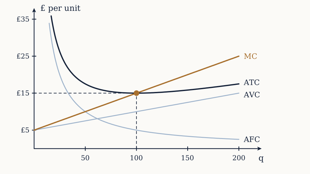
Four averages follow, and their notation is standard: average fixed cost $\mathrm{AFC}=F/q$, average variable cost $\mathrm{AVC}=V(q)/q$, average total cost $\mathrm{ATC}=C(q)/q$, and marginal cost $\mathrm{MC}=\mathrm{d}C/\mathrm{d}q$. Note that marginal cost contains no fixed component at all, since $F$ differentiates to zero. Marginal cost is a property of the variable input alone.

Marginal cost comes from marginal product

Cost curves are not free-standing; they are the production function seen through input prices. Suppose labour is the only variable input at wage $w$. Producing one more unit of output requires $1/{\mathrm{MP}}_L$ extra workers, each costing $w$, so

Marginal cost is the wage divided by the marginal product. That single equation explains the shape of every short-run cost curve in the subject: where marginal product rises, marginal cost falls, and where diminishing marginal returns set in, marginal cost turns upward. The U-shape of the cost curves is the inverted image of the hump in the product curves, not an independent assumption. By the same argument $\mathrm{AVC}=w/{\mathrm{AP}}_L$.

Example. The workshop from the previous lesson has $q=30L^2-L^3$ and pays £600 a week per worker. Find marginal cost at $L=10$ and at $L=18$.

The marginal product is $60L-3L^2$, which is 300 at $L=10$ and 108 at $L=18$. So marginal cost is $600/300=\pounds 2$ per unit and $600/108=\pounds 5.56$ per unit. Output at those two staffing levels is 2000 and 3888, so the firm's marginal cost has nearly tripled while its output has not quite doubled. That is diminishing returns expressed in pounds.

Now you. At what number of workers is this firm's marginal cost at its lowest, and what is it there?

The geometry of the cost curves

The relationship between marginal and average from the previous lesson reappears exactly, with cost in place of product. Differentiating $\mathrm{ATC}=C(q)/q$,

So average total cost falls while marginal cost is below it, rises while marginal is above it, and is stationary where they are equal. Marginal cost cuts average total cost at the minimum of average cost, and it does so from below. The same argument applies to average variable cost. This is not an empirical regularity or a drawing convention; it is a consequence of what an average is, and it will be doing serious work in the next two lessons.

Example. A firm has $C(q)=500+5q+0.05q^2$. Find the four cost measures at $q=50$, $q=100$ and $q=150$, and locate the minimum of average total cost.

Marginal cost is $\mathrm{MC}=5+0.1q$. At $q=50$: total cost is $500+250+125=\pounds 875$, so $\mathrm{AFC}=10$, $\mathrm{AVC}=7.50$, $\mathrm{ATC}=17.50$, and $\mathrm{MC}=\pounds 10$. Marginal is below average, so average is falling. At $q=100$: total cost is £1500, $\mathrm{ATC}=\pounds 15$, and $\mathrm{MC}=\pounds 15$. They are equal, so this is the minimum. At $q=150$: total cost is £2375, $\mathrm{ATC}=\pounds 15.83$, and $\mathrm{MC}=\pounds 20$; marginal is above average and average is climbing again. Confirming by calculus: $\mathrm{ATC}=500/q+5+0.05q$, and setting the derivative $-500/q^2+0.05$ to zero gives $q^2=10000$, so $q=100$.

Now you. A firm has $C(q)=800+4q+0.02q^2$. Find the output that minimises average total cost, and the value of average and marginal cost there.

One honest note about this example. Its average variable cost, $5+0.05q$, rises from the very first unit, so it has no U-shape. A U-shaped average variable cost requires a range over which marginal product is rising, which needs a cubic variable cost rather than a quadratic one. Textbook diagrams almost always draw the U; a great many real short-run cost functions look more like this one, with marginal cost roughly flat over normal operating ranges and turning up sharply near capacity.

The long run is an envelope

In the long run nothing is fixed, so the firm picks the plant as well as the output. Suppose it can build any of a family of plants, each with its own short-run cost curve. For any output it will use the plant that makes that output most cheaply, so the long-run average cost curve is the lower envelope of all the short-run curves: at each output it takes the smallest value any plant offers.

Two consequences follow. Long-run average cost is never above short-run average cost at the same output, because building the right plant is always an option. And the envelope touches each short-run curve at exactly one output, the one that plant is optimal for, which need not be that plant's own cheapest output.

Example. A firm can build a small plant with $C_1=500+0.05q^2$ or a medium one with $C_2=2000+0.0125q^2$. At what output should it switch, and what is average cost on either side?

Setting the totals equal: $500+0.05q^2=2000+0.0125q^2$, so $0.0375q^2=1500$ and $q=200$. At $q=100$ the small plant gives average cost $1000/100=\pounds 10$ against the medium plant's $2125/100=\pounds 21.25$, so small wins. At $q=400$ the small plant gives £21.25 and the medium gives £10, so medium wins. At the switch point both cost £2500, an average of £12.50 each.

Now you. A large plant costs $C_3=8000+0.003125q^2$. At what output does the firm switch from the medium plant to the large one?

Economies of scale, and how far they go

Long-run average cost falling with output is economies of scale; rising is diseconomies. The sources of the first were listed in the previous lesson: indivisibilities, specialisation, and the geometric fact that container volume grows faster than container surface. Diseconomies are mostly about management. Coordination, monitoring and information loss grow more than proportionally with the number of people who have to agree on something, and no technology has abolished that.

The scale at which average cost stops falling is the minimum efficient scale, and it is the single most useful number about an industry, because it sets how many firms the market can hold. A market whose total demand is ten times the minimum efficient scale can support ten efficient firms; one whose demand is twice it cannot support more than two. Structure follows from technology, which is why the market structure lessons come after this one rather than before.

The measured picture is less dramatic than the textbook diagram. Laurits Christensen and William Greene, studying United States electricity generation in 1976, found that scale economies had largely been exhausted by 1970, with most output produced by firms already operating on the flat part of the curve. Car assembly is usually put in the low hundreds of thousands of vehicles a year per plant, well below world demand, which is why the industry has many producers rather than one. Long-run average cost curves in practice tend to be L-shaped: falling sharply, then flat over a wide range, rather than U-shaped with a single sweet spot.

Cost falls with experience, not only with scale

One effect the whole apparatus of this lesson misses is that costs fall over time with cumulative production, independently of the current rate of output. T. P. Wright measured it on airframes in 1936 and found that each doubling of cumulative units built cut labour cost per unit by roughly 20 per cent. The same pattern has since been documented across semiconductors, wind turbines and photovoltaic modules, where the learning rate is also around 20 per cent per doubling and has held over more than four orders of magnitude of cumulative output.

This is a different axis from scale. Economies of scale are about output per year; learning is about output ever. A firm can sit at the same annual rate for a decade and still see its costs fall. Nothing in a static cost function represents this, and any argument about industrial policy that turns on infant industries is really an argument about learning curves rather than about scale.

The firm now has a cost function and knows what any output would cost. It still has no reason to pick one output rather than another, because nothing has yet been said about what the output sells for. Supplying that is the next lesson, and the answer depends entirely on how much market power the firm has.

A firm with a cost function still has no reason to prefer one output to another until something is said about what the output sells for.

The simplest possible assumption is that the firm cannot affect the price at all, and this lesson works out its consequences in full. The assumption is false of almost every real firm, which is exactly why it is worth doing first: it produces a benchmark against which market power can be measured, and the next three lessons are all measurements against it.

What price taking means

A firm is a price taker when its own output decision leaves the market price unchanged, so the demand curve facing it is horizontal at the going price. Sell one unit or a thousand, the price is the same, and try to charge a penny more and sales go to zero.

Four conditions are conventionally listed as sufficient for this. There are many buyers and many sellers, each small relative to the market. The product is homogeneous, so nobody has a reason to prefer one seller. Buyers and sellers know the prices on offer. And entry and exit are free in the long run, which does no work in the short run but everything in the long.

Note what these conditions actually deliver. Homogeneity plus information is what makes the individual demand curve horizontal, because a seller charging more is undercut by an identical product. Smallness is what makes the firm's output too little to move the market price. And note the honest point about the elasticity from three lessons ago: market demand for wheat is highly inelastic, while the demand curve facing one wheat farm is effectively perfectly elastic. Those are consistent, and confusing them is a standard error.

Nothing meets all four conditions exactly. Wheat, foreign exchange and standardised financial contracts come close. George Stigler pointed out in 1957 that the concept only became precise long after economists started using it, and its value is as a limiting case rather than a description.

Profit maximisation

Profit is revenue minus cost, $\pi (q)=R(q)-C(q)$. Differentiating and setting to zero,

Marginal revenue equals marginal cost. This is the general condition for any firm, competitive or not, and it is the marginal rule from the first lesson with revenue as the benefit. For a price taker, revenue is $R=pq$ with $p$ constant, so $\mathrm{MR}=p$ and the condition becomes

The second-order condition matters here and is usually skipped. A maximum requires ${\pi }^{\prime \prime }<0$, which for a price taker means ${\mathrm{MC}}^{\prime }(q)>0$: marginal cost must be rising at the chosen output. Where marginal cost is falling, $p=\mathrm{MC}$ locates a profit minimum, and the firm should move away from it in either direction. That is why only the upward-sloping part of the marginal cost curve is ever a supply curve, and it is also the first hint that a firm with continuously falling costs cannot be a price taker at all.

Example. A firm has $C(q)=500+5q+0.05q^2$ and the market price is £25. What does it produce, and what profit does it make?

Marginal cost is $5+0.1q$. Setting that equal to 25 gives $q=200$, and marginal cost is rising there, so it is a maximum. Revenue is $25\times 200=\pounds 5000$ and total cost is $500+1000+2000=\pounds 3500$, so profit is £1500. Equivalently, average total cost at 200 units is $3500/200=\pounds 17.50$, and profit is the margin times the quantity, $(25-17.50)\times 200=\pounds 1500$.

Now you. The same firm faces a price of £15. What does it produce, and what profit does it make?

When to keep operating at a loss

Suppose the price falls below average total cost, so the firm loses money. Shutting down is not automatically right, because in the short run the fixed cost is paid either way.

Compare the two options. Operating gives profit $pq-V(q)-F$. Shutting down gives $-F$. Operating is better when $pq-V(q)>0$, that is when $p>\mathrm{AVC}$. The shutdown condition is therefore a comparison with average variable cost, not average total cost, and the fixed cost drops out of it entirely, exactly as a cost common to both branches must.

Example. The same firm faces a price of £8. Should it produce, and what happens to its profit?

Setting $5+0.1q=8$ gives $q=30$. Revenue is £240, total cost is $500+150+45=\pounds 695$, so the loss is £455. Average variable cost at 30 units is $195/30=\pounds 6.50$, which is below the price of £8. So operating is right: shutting down would lose the full £500 of fixed cost, and producing loses only £455. The £45 difference is the contribution the output makes towards the fixed cost.

Now you. The price falls to £6. What should the firm do?

The long run differs because there are no fixed costs in it: every commitment can be ended. So the long-run exit condition compares price with average total cost, and a firm that cannot cover all its costs leaves.

From the firm to the industry

The firm's supply curve is therefore its marginal cost curve above average variable cost, and nothing at all below that. Rearranging $p=5+0.1q$ gives $q=10(p-5)$ for $p\ge 5$.

Market supply is the horizontal sum of the individual curves: at each price, add the quantities. Horizontal, not vertical, because the price is common and the quantities add. With $n$ identical firms, $Q=10n(p-5)$.

Example. One hundred such firms face market demand $Q=25000-500p$. Find the short-run equilibrium price, the industry quantity, each firm's output and its profit.

Industry supply is $Q=1000(p-5)=1000p-5000$. Setting supply equal to demand, $1000p-5000=25000-500p$, so $1500p=30000$ and $p=\pounds 20$. Industry output is 15,000 units and each firm makes 150. Checking against the firm: marginal cost at 150 is $5+15=\pounds 20$, matching the price. Each firm's total cost is £2375, so profit is $3000-2375=\pounds 625$.

Now you. Suppose 200 such firms are in the industry, facing the same demand curve. Find the equilibrium and each firm's profit.

Entry, exit, and the zero-profit result

Those two answers bracket the long run. With 100 firms there are profits, which attract entry; with 200 there are losses, which force exit. Entry shifts the industry supply curve right and drives the price down; exit does the reverse. Neither stops until economic profit is zero.

Zero profit requires $p=\mathrm{ATC}$. Profit maximisation requires $p=\mathrm{MC}$. Both hold only where $\mathrm{MC}=\mathrm{ATC}$, which the previous lesson established happens exactly at the minimum of average total cost. So the long-run competitive equilibrium has

For this firm that price is £15 and that output is 100 units. At £15 the market demands $25000-7500=17500$ units, so the industry settles at 175 firms each making 100 units. That number was not assumed anywhere; it fell out of the technology, which fixes the efficient scale, and the demand, which fixes how many such firms fit.

Three things are worth extracting from this. Each firm ends up at its own minimum average cost, so the industry's output is produced as cheaply as the technology allows. Price equals marginal cost, which the next lesson shows is the condition for efficiency. And economic profit is zero, meaning owners earn exactly what their resources would earn elsewhere, which is a statement about opportunity cost rather than about hardship.

The long-run industry supply curve is horizontal at £15 if input prices do not change as the industry expands, which is the constant cost case. If expansion bids up the price of a specialised input, minimum average cost rises with industry output and long-run supply slopes upward: that is the increasing cost case, and it is what makes long-run supply of anything using land or a scarce skill less than perfectly elastic.

What the model gets right and what it assumes away

Entry and exit are not theoretical. In the United States, roughly a tenth of employer firms are born and a comparable share die in a typical year, with the churn concentrated in retail, food service and construction, which are the industries closest to the assumptions here. The mechanism the model describes is visibly at work even though no market meets its conditions exactly.

Two assumptions do most of the load-bearing and deserve to be named. Free entry means entry at the same costs as incumbents, with no patent, licence, sunk investment or established brand in the way. William Baumol, John Panzar and Robert Willig showed in 1982 that this matters more than the number of firms: a market with two firms but genuinely free entry and costless exit behaves competitively, because the threat of entry disciplines price. Contestability, not headcount, is what the zero-profit argument needs.

And the whole apparatus assumes the firm has one product, one price, and no ability to be preferred by any buyer. Drop the last of those and the firm faces a downward-sloping demand curve of its own, which is the situation of nearly every real business. Before that, though, the competitive outcome needs to be evaluated rather than merely described: the next lesson asks what is good about $p=\mathrm{MC}$, and gets a sharper answer than might be expected.

Demand says what buyers will take at each price and supply says what sellers will offer, and the market price is the one number at which those two answers agree.

Marshall's scissors metaphor is the right one: asking whether demand or supply determines the price is like asking which blade of a pair of scissors cuts the paper. This lesson finds the crossing point, defines what each side gains from trading there, establishes the sense in which that quantity is the best one, and then breaks it with a tax to see what breaking it costs.

Equilibrium and the adjustment story

Take demand $Q_d=120-2p$ and supply $Q_s=3p-30$, both in units per week with $p$ in pounds. Setting them equal, $120-2p=3p-30$, so $5p=150$ and $p=\pounds 30$, with $Q=60$ units.

The claim that the market goes there needs an argument, and the standard one is about disequilibrium. At £40 supply is 90 and demand is 40, so 50 units go unsold, and sellers holding stock they cannot shift cut prices. At £20 demand is 80 and supply is 30, so buyers who cannot get the good bid the price up. Only at £30 does nobody have a reason to move. This is a story about incentives to change price rather than a theorem, and it can fail: markets with long production lags can oscillate around the equilibrium rather than converge to it, which is the cobweb model, and agricultural prices genuinely do this.

Comparative statics is the routine use of the model. A shift of one curve moves the equilibrium along the other, so the direction of the price and quantity changes identifies which curve moved. A bad harvest shifts supply left, raising price and cutting quantity. A fashion for a good shifts demand right, raising both. Price and quantity moving in opposite directions is the signature of a supply shift; in the same direction, a demand shift. That inference is the closest this apparatus gets to reading history off a price series, and it is also why the identification problem from the elasticity lesson is hard: without knowing which curve moved, the data say nothing about either.

Consumer and producer surplus

Trade makes both sides better off, and the areas on the diagram measure by how much. Jules Dupuit constructed the first such measure in 1844, while working out whether a bridge was worth building, and Marshall named it in 1890.

Read the demand curve as a marginal willingness to pay: the height at quantity $q$ is what the buyer of the $q$th unit would have paid at most. Everyone pays the market price, so each buyer's gain is the gap between their valuation and the price, and consumer surplus is the integral of that gap:

Geometrically it is the area below the demand curve and above the price. Similarly, the height of the supply curve at $q$ is the marginal cost of the $q$th unit, so producer surplus is the area above the supply curve and below the price, which equals revenue minus variable cost. Note that producer surplus is not profit: it exceeds profit by the fixed cost, since fixed costs never appear in a supply curve.

Example. For the market above, compute consumer and producer surplus at the equilibrium.

Inverting demand, $p=60-Q/2$, so the choke price is £60 and the demand curve meets the axis there. Consumer surplus is the triangle of height $60-30=\pounds 30$ and base 60 units, giving $\frac{12}{\times }60\times 30=\pounds 900$ a week. Inverting supply, $p=10+Q/3$, so the lowest price at which anything is supplied is £10, and producer surplus is $\frac{12}{\times }60\times 20=\pounds 600$. Total surplus is £1500.

Now you. A market has $Q_d=200-4p$ and $Q_s=4p-40$. Find the equilibrium and both surpluses.

Why the competitive quantity is the right one

Now the result that the rest of the course is measured against. Consider any quantity $q$ and ask whether producing one more unit raises total surplus. The buyer values it at $p_d(q)$, the demand curve height. It costs $p_s(q)$ to make, the supply curve height. The unit is worth making exactly when $p_d(q)>p_s(q)$, so surplus rises with output while demand lies above supply and falls once supply lies above demand. Total surplus is therefore maximised where the two curves cross, which is the competitive equilibrium.

Said in terms of the firm's condition, the competitive outcome has $p=\mathrm{MC}$, and price is marginal value while marginal cost is marginal cost, so the last unit produced is worth exactly what it costs. That is the whole content of the efficiency claim. Every unit whose value exceeds its cost gets made, and no unit whose cost exceeds its value does.

Three qualifications keep this from meaning more than it does, and all three become lessons later.

Total surplus counts a pound the same whoever receives it. A change that takes £100 from a poor buyer and gives £120 to a rich seller raises total surplus, and calling that an improvement is a normative judgement the model does not make and cannot support. Efficiency is a statement about the size of the pie only.

The demand curve measures willingness to pay, which is bounded by ability to pay. Somebody with no money has no willingness to pay for anything, and their needs do not appear on the diagram at all.

And the result assumes every cost and benefit falls on the two parties trading. When it does not, the supply curve is not marginal social cost and the whole argument fails, which is what the externalities lesson is about.

A tax drives a wedge

Put a tax of $t$ per unit on sellers. They now need $t$ more than before to supply any given quantity, so the price buyers pay and the price sellers receive differ by exactly $t$: $p_b-p_s=t$. Which side the tax is legally levied on makes no difference at all to the outcome, since the equations only contain the wedge. This is the irrelevance of statutory incidence, and it is one of the most robust and least believed results in the subject. Jonathan Gruber's study of the large payroll tax cuts in Chile between 1981 and 1986 found essentially full shifting into wages, exactly as the model says: who writes the cheque does not decide who bears the burden.

Example. The market $Q_d=120-2p$, $Q_s=3p-30$ faces a tax of £10 per unit. Find the two prices, the quantity, the revenue, and how the burden splits.

With $p_s=p_b-10$, supply becomes $Q_s=3(p_b-10)-30=3p_b-60$. Setting that equal to demand, $120-2p_b=3p_b-60$, so $5p_b=180$ and $p_b=\pounds 36$, $p_s=\pounds 26$, and $Q=48$. Buyers pay £6 more than before, sellers receive £4 less, so buyers bear 60 per cent of the tax. Revenue is $10\times 48=\pounds 480$ a week.

The 60 per cent is predictable from elasticities. At the original equilibrium, ${\epsilon }_d=-2\times 30/60=-1$ and ${\epsilon }_s=3\times 30/60=1.5$. The buyers' share is ${\epsilon }_s/({\epsilon }_s+|{\epsilon }_d|)=1.5/2.5=0.6$. The rule behind it is simple: the more inelastic side bears more of the tax, because being inelastic means having fewer alternatives to escape into.

Now you. The market $Q_d=200-4p$, $Q_s=4p-40$ faces a tax of £8 per unit. Find the two prices, the quantity, and the split.

Deadweight loss grows with the square of the tax

The tax cut output from 60 to 48. Those twelve units were worth more to buyers than they cost to make, and now they are not produced. Their lost surplus is the triangle between the two curves over the missing range, with height $t$ and base $\Delta Q$:

Here that is $\frac{12}{\times }10\times 12=\pounds 60$ a week. Check the accounting: consumer surplus falls from £900 to $\frac{12}{\times }48\times 24=\pounds 576$, and producer surplus from £600 to $\frac{12}{\times }48\times 16=\pounds 384$. The two losses sum to $324+216=\pounds 540$, of which £480 arrives as government revenue and £60 goes nowhere. That £60 is the deadweight loss, or Harberger triangle after Arnold Harberger's 1954 use of it.

The important structural fact is that $\Delta Q$ is itself proportional to $t$, so deadweight loss is proportional to $t^2$. Doubling a tax quadruples its excess burden. On this market $\Delta Q=1.2t$, so $\mathrm{DWL}=0.6t^2$.

Example. Confirm the square rule by computing the deadweight loss of a £20 tax on the same market.

Supply becomes $3p_b-90$, and $120-2p_b=3p_b-90$ gives $p_b=\pounds 42$, $p_s=\pounds 22$ and $Q=36$. Deadweight loss is $\frac{12}{\times }20\times 24=\pounds 240$, which is four times the £60 from the £10 tax, as $0.6\times 400$ requires. Revenue is $20\times 36=\pounds 720$.

Now you. Find the price, quantity, revenue and deadweight loss for a £30 tax on the same market, and compare the revenue with that of the £20 tax.

Two policy conclusions come straight out of the algebra. Since excess burden grows with the square of the rate, several small taxes on different goods cost less in total than one large tax raising the same money, which is the case for a broad base and low rates. And since deadweight loss depends on how much the quantity moves, taxing inelastic things is cheaper in efficiency terms, which is the Ramsey rule of 1927 and also, uncomfortably, an argument for taxing necessities.

Floors and ceilings

A price ceiling below equilibrium creates excess demand, and a price floor above it creates excess supply. The surplus arithmetic is the same as for a tax except that no revenue is raised, so the whole reduction in trade is lost, and it is worse still if the units that do get traded are not the ones with the highest value or the lowest cost.

Rent control is the standard case and the evidence is more interesting than either side usually admits. Rebecca Diamond, Tim McQuade and Franklin Qian studied San Francisco's 1994 extension of rent control to small multi-family buildings and found that it delivered substantial benefits to the tenants covered, who were significantly more likely to stay in the city, while landlords responded by converting and redeveloping properties enough to cut the rental housing supply of affected buildings by about 15 per cent, raising rents city-wide. Both effects are real, they fall on different people, and the surplus arithmetic on its own cannot say which matters more. That is exactly the limit of this apparatus.

The efficiency benchmark is now established and one way of breaking it, taxation, has been measured. The next three lessons break it in a more fundamental way, by dropping the assumption that firms take the price as given.

Every result in the previous lesson rested on firms taking the price as given, and this lesson drops that single assumption and keeps everything else.

A monopoly is a market with one seller and no close substitute. What makes it a different problem is not size or wickedness but the shape of the demand curve the firm faces: it is the market demand curve, sloping downwards, so selling more requires charging less. That one change propagates through the whole analysis and produces a quantity below the efficient one, which is the first genuine failure of the competitive benchmark.

Where a monopoly comes from

Monopoly needs a barrier to entry, otherwise the profits attract competitors and the situation ends. Four kinds are worth distinguishing.

Legal barriers are the commonest and the most deliberate. A patent grants exclusive rights for twenty years from filing under the international agreement of 1994, on the explicit argument that temporary monopoly is the price of getting the invention at all. Copyrights, broadcast licences and taxi medallions do the same thing with less justification.

Control of a scarce input is the classic private route. De Beers held roughly 80 per cent of world rough diamond supply for much of the twentieth century by buying up production and stockpiling it, and its share fell below half in the 2000s once Russian, Australian and Canadian output found other channels. That trajectory is the normal one: input monopolies are eroded by discovery.

Natural monopoly arises when one firm can supply the whole market more cheaply than two can, which happens whenever average cost is still falling at the scale of total demand. Water distribution, electricity transmission and rail track are the standard examples, and this case gets a section of its own below because it cannot be fixed by encouraging entry.

Network effects make a product more valuable the more people use it, so an early lead compounds. This is the modern case and it is genuinely different from the others, since the barrier is created by the customers rather than by the firm.

Marginal revenue lies below price

Here is the whole of monopoly in one derivation. Revenue is $R=p(q)q$, where $p(q)$ is inverse demand. Differentiate with the product rule:

The first term is the money from the extra unit. The second is negative, because selling the extra unit requires cutting the price on every unit already being sold. A price taker has $\mathrm{d}p/\mathrm{d}q=0$ and the second term vanishes, which is why $\mathrm{MR}=p$ there. For anyone else marginal revenue is strictly below price.

Factor out $p$ and the elasticity appears:

This is worth reading carefully. If demand is inelastic, $|\epsilon |<1$, then $1+1/\epsilon$ is negative and marginal revenue is negative: selling more actually reduces revenue. Since costs are positive, a monopolist never operates on the inelastic part of its demand curve. It would raise price, sell less, earn more and spend less. Any firm found pricing where demand is inelastic is either not a monopolist or not maximising.

For linear inverse demand $p=a-bq$, revenue is $aq-b{q}^2$ and marginal revenue is $a-2bq$: the same intercept and twice the slope. That doubling is worth memorising, since it makes every linear monopoly problem a two-line calculation.

The monopoly output

Profit maximisation is $\mathrm{MR}=\mathrm{MC}$, exactly as for any firm. What differs is that marginal revenue is not the price, so the price ends up above marginal cost.

Example. A monopolist faces $p=100-2q$ and has $C(q)=100+20q$. Find its output, price and profit, compare with the competitive outcome, and compute the deadweight loss.

Marginal revenue is $100-4q$ and marginal cost is £20. Setting them equal, $100-4q=20$, so $q=20$ and $p=100-40=\pounds 60$. Profit is $60\times 20-(100+400)=\pounds 700$.

A competitive industry with the same costs would produce where $p=\mathrm{MC}$: $100-2q=20$ gives $q=40$ at a price of £20. So the monopolist sells half as much at three times the price. The deadweight loss is the triangle between demand and marginal cost over the missing 20 units, $\frac{12}{\times }(60-20)\times (40-20)=\pounds 400$ a week. Consumer surplus falls from $\frac{12}{\times }40\times 80=\pounds 1600$ to $\frac{12}{\times }20\times 40=\pounds 400$, so consumers lose £1200, of which £800 is transferred to the firm as profit and £400 is destroyed.

Now you. A monopolist faces $p=120-3q$ with $C(q)=200+30q$. Find output, price, profit and deadweight loss.

The markup rule

Substituting $\mathrm{MR}=p(1+1/\epsilon )$ into $\mathrm{MR}=\mathrm{MC}$ and rearranging gives the result in its most useful form:

The left side is the Lerner index, defined by Abba Lerner in 1934 as the fraction of price that is markup over marginal cost. It is the standard measure of market power, running from 0 for a price taker to 1 as elasticity approaches zero. The result says the markup is determined entirely by the elasticity of demand at the chosen point, and by nothing else: not by cost, not by firm size, not by how many competitors are visible.

In the worked example, price is £60 and marginal cost £20, so the Lerner index is $40/60=0.667$. The elasticity at that point is $(-1/2)(60/20)=-1.5$, and $-1/(-1.5)=0.667$. The two agree, as they must.

The rule also explains why monopolists do not charge "as much as possible". There is no such quantity. The firm charges the amount that makes the elasticity consistent with its costs, which for a low-cost firm facing elastic demand can be a very modest markup.

A monopolist has no supply curve

This sounds like a technicality and is not. A supply curve answers "how much would you produce at price $p$", and that question is meaningless for a monopolist, because it chooses the price rather than reading it off the market. Its output depends on the whole shape of demand, not on one point of it, and two different demand curves passing through the same price and quantity can produce different monopoly outputs. The supply curve is an artefact of price taking, and dropping price taking dissolves it.

Natural monopoly, and the trouble with regulating it

When average cost falls over the whole range of demand, the efficient number of firms is one, and the competitive prescription $p=\mathrm{MC}$ becomes a trap. With falling average cost, marginal cost lies below average cost everywhere, so a firm charging marginal cost loses money on every unit and cannot survive without a subsidy.

Example. A water utility faces $p=70-0.5q$ and has $C(q)=1600+10q$. Find the unregulated monopoly outcome, what happens under marginal cost pricing, and what price covers costs exactly.

Unregulated: $\mathrm{MR}=70-q=10$, so $q=60$ and $p=\pounds 40$, with profit $2400-2200=\pounds 200$.

Marginal cost pricing: $p=\pounds 10$ gives $q=120$, revenue £1200 against costs of $1600+1200=\pounds 2800$, a loss of £1600. That loss is exactly the fixed cost, which is what constant marginal cost guarantees. The efficient quantity is unfinanceable at the efficient price.

Average cost pricing: set $70-0.5q=1600/q+10$, which rearranges to $q^2-120q+3200=0$ with roots 40 and 80. The regulator wants the larger one, so $q=80$ at $p=\pounds 30$, where average cost is $1600/80+10=\pounds 30$ exactly. The firm breaks even and output is two thirds of the efficient level.

Now you. For that utility, compute the deadweight loss under average cost pricing and under unregulated monopoly.

Average cost pricing, or rate-of-return regulation, is what most utility regulators actually do, and it has a well documented side effect. Harvey Averch and Leland Johnson showed in 1962 that a firm allowed a fixed return on its capital base has an incentive to enlarge that base, choosing a more capital-intensive method than cost minimisation would pick. Frank Ramsey's 1927 alternative, spreading the fixed cost across products in inverse proportion to their elasticities, minimises the deadweight loss subject to breaking even, and is used in rail and postal pricing.

Price discrimination

A single price leaves money on the table: buyers who would have paid more get a surplus, and buyers who would have paid a little above marginal cost are not served at all. Price discrimination is charging different prices to different buyers for reasons unrelated to cost. It requires market power, some way of telling buyers apart, and a way to prevent resale.

First degree, or perfect, discrimination charges each buyer their full willingness to pay. Output rises to the efficient level, because every unit worth more than marginal cost now gets sold, and the deadweight loss vanishes entirely. All of the surplus goes to the seller. This is the sharpest illustration in the subject that efficiency and fairness are separate axes.

Second degree offers a menu and lets buyers sort themselves: bulk discounts, first and standard class, advance purchase fares. The seller does not know who is who, so the menu has to be designed so that each type prefers the option intended for it.

Third degree charges different prices to identifiable groups: student tickets, senior discounts, regional pricing. Here the arithmetic is clean, because the firm simply runs a separate monopoly problem in each market with the same marginal cost.

Example. A firm with constant marginal cost £20 sells in two separated markets, $p_1=100-2q_1$ and $p_2=80-q_2$. Find its prices, and check them against the elasticities.

In market 1, $100-4q_1=20$ gives $q_1=20$ and $p_1=\pounds 60$. In market 2, $80-2q_2=20$ gives $q_2=30$ and $p_2=\pounds 50$. Total profit is $1200+1500-1000=\pounds 1700$. The elasticities are $-1.5$ in market 1 and $-1.67$ in market 2, so the lower price goes to the more elastic market, exactly as the markup rule requires. Forced to charge one price, the firm would set £53.33 and earn £1666.67, so discrimination is worth £33.33 a week to it.