Differential Equations

Almost every quantitative law in science says something about a rate of change rather than about a value, so the thing it pins down is a function and not a number.

Ernest Rutherford and Frederick Soddy found in 1902 that a radioactive sample loses atoms at a rate proportional to how many it still has. That sentence is not a formula for the number of atoms. It is a constraint linking the unknown function $N(t)$ to its own derivative, $\frac{dN}{dt}=-kN$, and the work of extracting $N(t)$ from it is what this course is about. Newton's second law is the same kind of statement, one derivative further along: force is mass times acceleration, and acceleration is the second derivative of position, so every mechanical problem arrives as a constraint on $x(t)$ and $x^{\prime \prime }(t)$ rather than as a recipe for $x$.

This lesson assumes the derivative rules and definite integration from the previous course, and nothing else. It sets up the vocabulary, then shows the one thing that can always be done to a differential equation even when it cannot be solved.

A law of change is an equation for a curve

A differential equation is an equation relating an unknown function to one or more of its derivatives. A solution is a function that satisfies it on some interval, and the word "some" is doing real work there, as the end of the lesson shows.

The distinction from ordinary algebra is worth making slowly, because it is where beginners lose their footing. Solving $x^2-5x+6=0$ produces two numbers, $2$ and $3$, and checking them is arithmetic. Solving $y^{\prime }=2y$ produces a family of functions, $y=C{e}^{2t}$ for every constant $C$, and checking one is differentiation. The unknown lives in a space of functions, so the answer is a curve, or rather infinitely many curves, one through every point of the plane.

We restrict to ordinary differential equations, where the unknown depends on one variable, almost always time. If the unknown depends on several variables, the derivatives are partial and the equation is a partial differential equation: the heat equation and the wave equation are the standard examples, and they need machinery beyond this course. Everything here is one independent variable, which is enough for mechanics, circuits, chemical kinetics and population models.

Order, linearity, and why the labels stick

Two labels decide which method will work, so they are worth fixing before any method exists.

The order is the highest derivative that appears. $\frac{dN}{dt}=-kN$ is first order. The spring equation $m{x}^{\prime \prime }+c{x}^{\prime }+kx=0$ is second order. Order is not a matter of taste: it counts how much information you must supply to select one solution out of the family, and it is why a projectile needs both a launch position and a launch velocity while a decaying sample needs only its starting mass.

An equation is linear if the unknown and its derivatives appear only to the first power, never multiplied together, and never inside a function like $\sin$ or a square root. The general linear equation of second order is

where the coefficients may be any functions of $t$ at all. Linearity is a statement about how $y$ enters, not about how $t$ enters: $y^{\prime }+t^{2}y=\cos t$ is linear, and $y^{\prime }=y^2$ is not. If $g(t)$ is zero the linear equation is called homogeneous, and if not, the term $g$ is the forcing.

Linear equations are the ones with a complete theory, because solutions can be added: if $y_1$ and $y_2$ both solve a homogeneous linear equation, so does $y_1+y_2$. Try that on $y^{\prime }=y^2$. With $y_1=-1/t$ and $y_2=-1/(t+1)$, both genuine solutions, the sum satisfies nothing at all. Nonlinear equations lose superposition, and with it most of the algebra, which is why the second half of this course spends its effort on reading nonlinear solutions rather than writing them.

Verifying a solution

Checking a candidate needs no theory: differentiate it, substitute, and see whether the two sides agree for every $t$ in the interval, not just at one point.

Example. Show that $y=3e^{2t}-2e^{-t}$ solves $y^{\prime \prime }-y^{\prime }-2y=0$, and find $y(0)$ and $y^{\prime }(0)$.

Differentiating, $y^{\prime }=6e^{2t}+2e^{-t}$ and $y^{\prime \prime }=12e^{2t}-2e^{-t}$. Substituting,

The $e^{2t}$ terms give $12-6-6=0$ and the $e^{-t}$ terms give $-2-2+4=0$, so the left side is identically zero and the candidate is a solution. At $t=0$, $y(0)=3-2=1$ and $y^{\prime }(0)=6+2=8$.

Now you. Show that $y=C_1{e}^{3t}+C_2{e}^{-2t}$ solves $y^{\prime \prime }-y^{\prime }-6y=0$ for every pair of constants, and find $y(0)$ and $y^{\prime }(0)$ in terms of $C_1$ and $C_2$.

Verification is cheap and solving is expensive, which is a lopsidedness worth exploiting. Guessing a form, substituting it, and letting the equation fix the constants is a legitimate and heavily used method, and it is exactly how the constant-coefficient theory later in this course is built.

Why solutions come in families

The simplest differential equation is $y^{\prime }=f(t)$, whose solution is an antiderivative of $f$. There is never exactly one: antiderivatives differ by a constant, so the answer is a family $y=F(t)+C$, and that single arbitrary constant is the residue of everything the equation does not know. The equation constrains the slope at every instant and says nothing about where the curve starts.

That generalises. An equation of order $n$ has a general solution carrying $n$ arbitrary constants, and a particular solution is one member of the family with the constants fixed. The count matches the order because integrating $n$ times introduces $n$ constants, and it is the reason order is the first thing to identify.

To select a member you supply extra data. An initial value problem gives the value of the function and of its first $n-1$ derivatives at one instant $t_0$. For a second order equation that is a position and a velocity, which is precisely the state Newtonian mechanics says determines a trajectory. Supplying data at two different instants instead, such as $y(0)=0$ and $y(1)=0$, makes it a boundary value problem, which behaves quite differently: such problems can have no solution or infinitely many, and this course stays with initial conditions.

Example. The general solution of $y^{\prime \prime }+4y=0$ is $y=A\cos 2t+B\sin 2t$, which you can check by substituting. Solve the initial value problem with $y(0)=3$ and $y^{\prime }(0)=8$, and give the amplitude of the resulting oscillation.

Setting $t=0$ in $y$ gives $y(0)=A=3$. Differentiating, $y^{\prime }=-2A\sin 2t+2B\cos 2t$, so $y^{\prime }(0)=2B=8$ and $B=4$. The particular solution is $y=3\cos 2t+4\sin 2t$. Combining the two terms into a single sinusoid gives amplitude $\sqrt{A^2+B^2}=\sqrt{9+16}=5$, so the motion runs between $-5$ and $5$.

Now you. For the same equation, solve the initial value problem with $y(0)=-2$ and $y^{\prime }(0)=12$, and give the amplitude.

Building the equation from the words

Most of the difficulty in applying this subject is not solving the equation but writing it down, and writing it down is always the same move: express the rate of change of the quantity as the sum of everything adding to it minus everything removing it.

Take the decay law. In one year a radiocarbon sample loses a fixed fraction of whatever it has, so $\frac{dN}{dt}=-kN$, and the constant is fixed by the measured half-life of $5730$ years for carbon-14. Setting $N=N_0/2$ in the solution $N=N_0{e}^{-kt}$ gives $k=\ln 2/5730=1.210\times {10}^{-4}$ per year. That number then dates anything organic: a sample holding $78$ per cent of its original carbon-14 has been dead for $\ln (1/0.78)/k=2054$ years.

Take a falling body with air resistance. Gravity pulls down with force $mg$, drag opposes motion with a force that at everyday speeds is close to proportional to $v^2$, and Newton's law assembles them into

first order, nonlinear because of the square, and already interesting before it is solved: whenever $b{v}^2$ reaches $mg$ the derivative vanishes and the speed stops changing. That terminal speed is $\sqrt{mg/b}$, read off the equation itself without any solving. A skydiver in a spread posture has $m/b$ near $300$ m, giving $\sqrt{300\times 9.81}=54$ m s⁻¹, or about $195$ km h⁻¹, which is the figure the sport quotes.

Take a mixing tank. Brine at $c_{\text{in}}$ kilograms per cubic metre enters at $q$ cubic metres per minute, the tank holds $V$ cubic metres and is stirred so its concentration is uniform, and the outflow matches the inflow. The salt mass $S$ changes at the rate it enters minus the rate it leaves, $\frac{dS}{dt}=q{c}_{\text{in}}-\frac{q}{V}S$: first order and linear, and the model for every stirred reservoir from a chemical reactor to a lake.

Direction fields: the family without the formula

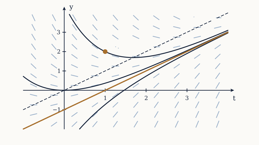
Here is the move that makes an unsolvable equation useful. A first order equation $y^{\prime }=f(t,y)$ hands you the slope of the solution at every point of the plane before you know any solution. Draw a short segment of that slope at each of a grid of points and you have a direction field: solutions are exactly the curves that stay tangent to it everywhere, and the eye assembles them from the picture.

Consider $y^{\prime }=t-y$. At the point $t=1$, $y=2$ the slope is $1-2=-1$. On the line $y=t$ every slope is zero, so solutions crossing that line do so horizontally. Above it slopes are negative and below it positive, so every solution is pushed towards the line from both sides. The line itself is nearly a solution: trying $y=t-1$ gives $y^{\prime }=1$ and $t-y=1$, so it is a solution exactly. The picture says that whatever a solution does early on, it ends up hugging $y=t-1$, and this is right: the general solution turns out to be $y=t-1+C{e}^{-t}$, and the $C{e}^{-t}$ term dies.

A curve on which the slope takes one fixed value is an isocline, and sketching a few is the fast way to draw a field by hand. For $y^{\prime }=t-y$ the isoclines are the straight lines $t-y=m$, one per slope $m$.

Example. For $y^{\prime }=y(1-y)$, find the slope at $y=0.5$, at $y=2$ and at $y=1$, and say what a solution starting at $y(0)=0.5$ does.

The slopes are $0.5\times 0.5=0.25$, then $2\times (1-2)=-2$, then exactly $0$. Since $f$ does not involve $t$, the slope depends only on the height, so each horizontal line carries a single slope. The lines $y=0$ and $y=1$ carry slope zero and are constant solutions. Between them the slope is positive, so a solution starting at $0.5$ rises, and since it can never cross the constant solution at $y=1$, it approaches $1$ from below without reaching it. Above $y=1$ slopes are negative, so those solutions fall to $1$ as well.

Now you. For $y^{\prime }=2-y$, give the slope at $y=0$, $y=2$ and $y=5$, and say what happens to a solution starting at $y(0)=5$.

What is actually solvable

An honest course says early what its methods will not reach. Almost every differential equation you can write down has no solution expressible in elementary functions. $y^{\prime }=t^2+y^2$ is about as simple as an equation gets, and its solutions require Bessel functions; $y^{\prime }=e^{-t^2}+y$ pulls in the error function immediately. This is not a gap in the textbooks. It is the same fact as most integrals having no elementary antiderivative, since integration is the special case $y^{\prime }=f(t)$.

So the subject has three tools rather than one, and they will be used throughout. Exact solution, where a formula exists and is worth having. Qualitative analysis, which reads the long-term behaviour off the equation itself, as the terminal speed and the direction field did above. Numerical solution, which produces a table of values to whatever accuracy is paid for. A good answer often uses all three: the numerics give the curve, the qualitative argument says the curve is believable, and the exact solution of a simplified version says what controls it.

Solutions also have limited lifetimes. $y^{\prime }=y^2$ with $y(0)=1$ has the solution $y=1/(1-t)$, which is perfectly well behaved near $t=0$ and infinite at $t=1$, even though the equation itself shows no sign of trouble there. A differential equation is a local statement, and asking where its solutions stop existing is a real question, taken up in a later lesson.

The next step is the first class of equations that yields completely. When the right side factors into a function of $t$ times a function of $y$, the variables can be separated and both sides integrated, which turns the decay law, the cooling law and the logistic curve into three lines of calculus each.

The previous lesson could draw the family of solutions to a first order equation without solving it, and this one solves a genuine class of them outright.

The class is narrow but it contains most of the standard models: radioactive decay, drug clearance, cooling, dissolution, and population growth against a limit. What they share is that the rate of change factors, with everything depending on time in one bracket and everything depending on the unknown in another. When that happens, calculus alone finishes the job.

The factoring that makes integration possible

An equation is separable if it can be written

The method is to divide by $h(y)$, multiply by $dt$, and integrate both sides. That description is a mnemonic rather than an argument, since $dt$ is not a quantity to be multiplied by, so here is the argument. Divide by $h(y)$ to get

and integrate both sides with respect to $t$. On the right that gives $\int g(t)dt$. On the left, the integrand is exactly of the form $F^{\prime }(y)y^{\prime }$ with $F$ an antiderivative of $1/h$, so the chain rule identifies it as the derivative of $F(y(t))$, and by substitution $\int \frac{1}{h(y)}\frac{dy}{dt}dt=\int \frac{dy}{h(y)}$. So

which is the mnemonic, now justified. Only one constant is needed, since the two would merge. What comes out is a relation between $y$ and $t$, not necessarily a formula for $y$, and that distinction matters below.

Example. Solve $\frac{dy}{dt}=ty$ with $y(0)=3$.

Separating, $\frac{dy}{y}=tdt$, so $\ln |y|={\frac{12}{t}}^2+C$ and $|y|=e^C{e}^{t^2/2}$. Absorbing the sign and the exponential of the constant into one constant $A$, the general solution is $y=A{e}^{t^2/2}$. The initial condition gives $A=3$, so $y=3e^{t^2/2}$. Checking: $y^{\prime }=3t{e}^{t^2/2}=ty$, as required.

Now you. Solve $\frac{dy}{dt}=y\cos t$ with $y(0)=2$.

The solutions that division destroys

Dividing by $h(y)$ is only legal where $h(y)$ is not zero, and every root of $h$ is a constant solution that the method throws away. If $h(y_0)=0$ then the constant function $y\equiv y_0$ has zero derivative and satisfies the equation exactly, yet it can never appear in the family produced by separating, because the very first step divided by zero to get there.

For $y^{\prime }=y(1-y)$ the roots are $y=0$ and $y=1$, and both are genuine solutions that must be added back by hand. Sometimes the lost solution reappears as a limiting case of the constant: for $y^{\prime }=ky$ the family $y=A{e}^{kt}$ includes $y\equiv 0$ at $A=0$, even though the derivation assumed $y\ne 0$. Sometimes it does not, and then the general solution is genuinely incomplete without it. Check the roots of $h$ every time; it costs one line and it is the standard way to lose half an answer.

Decay, growth and half-lives

The equation $\frac{dy}{dt}=ky$ says the rate of change is proportional to the amount present, and separating gives $y=y_0{e}^{kt}$. Negative $k$ is decay, positive is unconstrained growth. What makes the model useful is that $k$ is rarely quoted directly: what is measured is a half-life $t_{1/2}$, the time for the amount to halve, and setting $y=y_0/2$ gives $e^{k{t}_{1/2}}=\frac{12}{}$, so $k=-\ln 2/t_{1/2}$.

Caffeine leaves the bloodstream by first order kinetics with a half-life near $5$ hours in a typical adult. So $k=-\ln 2/5=-0.1386$ per hour, and a $200$ mg dose falls to $95$ mg after $t=\ln (200/95)/0.1386=5.4$ hours. The same arithmetic dates a bone from its carbon-14, sizes a shielding delay from a reactor isotope, and sets the dosing interval of a drug. The characteristic quantity is $1/|k|$, the time constant, after which the amount has fallen by a factor of $e$; a half-life is $\ln 2=0.693$ time constants.

The honest limit is that pure exponential growth is a statement about a system with unlimited resources, and no real population has those. It is the first term of a better model, not the model.

Newton's law of cooling, fitted to a real mug

A body at temperature $T$ in surroundings at $T_s$ loses heat at a rate roughly proportional to the excess temperature, which gives

Separating with $u=T-T_s$, which has the same derivative as $T$ since $T_s$ is constant, gives $u=u_0{e}^{-kt}$, so

Every cooling curve is the same shape: the excess over ambient decays exponentially, and the temperature approaches the room's, never crossing it.

Example. Coffee at $90$ °C stands in a room at $20$ °C. After $5$ minutes it reads $70$ °C. When will it reach $45$ °C?

The excess starts at $70$ degrees and is $50$ degrees after five minutes, so $50=70e^{-5k}$ and $k=\frac{15}{\ln }(70/50)=0.0673$ per minute. Drinking temperature at $45$ °C is an excess of $25$ degrees, so $25=70e^{-kt}$ and $t=\ln (70/25)/0.0673=15.3$ minutes. As a check, the prediction at ten minutes is $20+70e^{-0.673}=55.7$ °C, which is the same fall of $70$ to $50$ per cent applied twice.

Now you. Soup at $95$ °C sits in a room at $22$ °C and is at $65$ °C after $10$ minutes. When does it reach $40$ °C?

The law is an approximation, valid when the excess temperature is small enough that radiation, which goes as the fourth power of absolute temperature, is not dominant, and when the body is well stirred or thin enough to have one temperature at all. For a mug of coffee at kitchen temperatures both hold well enough that the fit above is good to a degree or so over half an hour.

Implicit solutions and the interval they live on

Separation produces a relation, and there is no guarantee that the relation can be solved for $y$. Take $\frac{dy}{dt}=-\frac{t}{y}$ with $y(0)=3$. Separating gives $ydy=-tdt$, so ${\frac{12}{y}}^2=-{\frac{12}{t}}^2+C$ and

a circle. That is a perfectly good implicit solution, and it says more clearly than any formula what the solutions look like. Made explicit, $y=\sqrt{9-t^2}$, taking the positive root because $y(0)=3$, and now the trouble is visible: the solution exists only for $-3<t<3$. At the ends the circle has a vertical tangent, the derivative is infinite, and the solution simply stops. Nothing in the original equation announced the number $3$; it came from the initial condition. The interval of existence of a solution can depend on where the solution starts, which never happens for the linear equations of the next lesson.

Some separable equations lead to integrals that need the techniques of the previous course. $\frac{dy}{dt}=\frac{y^2-1}{2}$ separates to $\int \frac{2dy}{(y-1)(y+1)}=\int dt$, a partial fractions problem, and others lead to integrals with no elementary form at all, at which point separation has converted a differential equation into a definite integral to be done numerically. That is still progress.

The logistic equation

Exponential growth fails because it ignores the resource limit. Model the limit in the crudest way that could work: let the per-capita growth rate fall linearly to zero as the population $P$ approaches a carrying capacity $K$. The per-capita rate is $\frac{1}{P}\frac{dP}{dt}$, so the assumption is $\frac{1}{P}\frac{dP}{dt}=r(1-\frac{P}{K})$, giving the logistic equation

published by Pierre-François Verhulst in 1838. It is separable and nonlinear. Separating and using partial fractions on $\frac{1}{P(1-P/K)}=\frac{1}{P}+\frac{1/K}{1-P/K}$ gives $\ln P-\ln (1-P/K)=rt+C$, so $\frac{P}{1-P/K}=A{e}^{rt}$, and solving for $P$,

The behaviour is the S-curve: growth is nearly exponential at rate $r$ while $P\ll K$, slows as the bracket shrinks, and levels off at $K$. The steepest point is where $\frac{dP}{dt}$ is largest, and since that is a downward parabola in $P$ with roots at $0$ and $K$, the maximum is at $P=K/2$, exactly half the capacity, at which the growth rate is $rK/4$.

Example. A lake is stocked with $100$ fish. The population grows logistically with $r=0.03$ per year and $K=1000$. When does it reach $500$?

Half capacity is reached when the denominator is $2$, that is when $(\frac{1000}{100}-1)e^{-rt}=1$, so $9e^{-0.03t}=1$ and $t=\ln 9/0.03=73.2$ years. That is also the moment of fastest growth, at $rK/4=7.5$ fish per year.

Now you. A population starts at $50$ with $r=0.05$ per year and $K=800$. When does it reach $400$?

Raymond Pearl and Lowell Reed fitted a logistic to the United States census in 1920 and obtained $K=197.3$ million, $r=0.0313$ per year, and half capacity in 1914. Against the census the fit is remarkable: it predicts $77.3$ million for 1900 against a measured $76.2$, and $107.9$ million for 1920 against $106.0$. It is also wrong in the way models of this sort are always wrong. The United States passed $197$ million in 1967 and kept going, because immigration and changing fertility are not in the model, and by 2020 the fit predicts $190$ million against an actual $331$. A logistic fit measures the growth pattern of the period it was fitted to, and its extrapolated $K$ is a summary of that period rather than a property of the country.

Where separation runs out

Separation needs the right side to factor, and most equations do not. Consider a stirred tank whose inflow concentration varies during the day, or a capacitor charged from a mains supply. Both give equations of the shape

with $g$ not constant, and there is no way to write $g(t)-p(t)y$ as a product of a function of $t$ and a function of $y$. Even the simplest instance, $y^{\prime }=t+y$, resists. Yet these equations are linear, which the logistic equation is not, and linear equations are supposed to be the easy ones.

They are, once the right trick is found. The next lesson finds it by asking what could be multiplied through the equation to make the left side the derivative of a single product, and the answer solves every first order linear equation there is.

Separation failed on equations as simple as $y^{\prime }=t+y$, and those are exactly the equations that describe a system being driven from outside.

A first order linear equation is one where the unknown and its derivative appear only to the first power and never multiplied together, so it can always be arranged as

with $p$ the coefficient and $g$ the forcing. Separation needs the right side to factor as a function of $t$ times a function of $y$, and $g(t)-p(t)y$ does not factor unless $g$ is constant or zero. This lesson finds the method that does work, and it works for every equation of this shape, whatever $p$ and $g$ are.

What we would like the left side to be

The whole difficulty is that $y^{\prime }+py$ is a sum of two unrelated-looking things. If instead the left side were the derivative of a single product, the equation could be integrated on sight, because the fundamental theorem would undo it in one step.

So demand it. Multiply the whole equation by an as-yet-unknown positive function $\mu (t)$:

and ask what $\mu$ would make the left side exactly $(\mu y{)}^{\prime }$. By the product rule $(\mu y{)}^{\prime }=\mu y^{\prime }+{\mu }^{\prime }y$, so the two agree for all $y$ precisely when

That is a separable equation for $\mu$, and we can already solve it: $\mu =e^{\int pdt}$. No constant of integration is needed, since any constant multiple of $\mu$ works equally well and would cancel later. This $\mu$ is the integrating factor, and it exists for every $p$ that can be integrated at all.

With it, the equation reads $(\mu y{)}^{\prime }=\mu g$, so integrating both sides,

That formula solves the entire class. It is worth remembering the derivation rather than the formula, because in practice you compute $\mu$, write the left side as a derivative, and integrate, which is less error-prone than substituting into a memorised expression.

Notice what has happened structurally. The single constant $C$ enters the answer multiplied by $1/\mu =e^{-\int pdt}$, and everything else comes from the forcing. Every first order linear equation therefore has a solution of the form "one particular response to the forcing, plus a constant times a decaying (or growing) function that remembers the initial condition". That split runs through the rest of the course.

Example. Solve $t{y}^{\prime }+2y=4t^2$ with $y(1)=2$, for $t>0$.

First put it in standard form by dividing by $t$: $y^{\prime }+\frac{2}{t}y=4t$. Then $\int pdt=\int \frac{2}{t}dt=2\ln t$, so $\mu =e^{2\ln t}=t^2$. Multiplying through,

Integrating, $t^{2}y=t^4+C$, so $y=t^2+C/t^2$. The condition $y(1)=2$ gives $1+C=2$, so $C=1$ and $y=t^2+1/t^2$. At $t=2$ that is $4.25$. Checking the original equation at any $t$ is a two-line differentiation, and it holds.

Now you. Solve $y^{\prime }-\frac{y}{t}=t$ with $y(1)=3$, for $t>0$.

Transient and steady state

Take the commonest case, constant $p=1/\tau$ and constant forcing $g$. The integrating factor is $e^{t/\tau }$, and the solution is

Two pieces, with quite different characters. The constant $g\tau$ is the steady state: it is what the equation settles to, and it depends only on the forcing and the coefficient, not on where the system started. The exponential is the transient: it carries the whole memory of the initial condition and decays with time constant $\tau$, reaching $1/e$ of its starting size after $\tau$, and under one per cent after $5\tau$.

This is why identical devices with different histories end up behaving identically, and why the time constant, rather than the initial condition, is what an engineer quotes. It also explains the earlier direction field for $y^{\prime }=t-y$, whose solutions all approached the line $y=t-1$: that line is the response to the forcing $g(t)=t$, and the $C{e}^{-t}$ that distinguishes one solution from another is the transient.

Charging a capacitor

A resistor $R$ in series with a capacitor $C$ across a source $V$ obeys Kirchhoff's voltage law: the source equals the drop across the resistor plus the voltage on the capacitor. With $i=C\frac{dv}{dt}$ the current through both,

which is the standard form with $\tau =RC$. Its solution from $v(0)=0$ is $v=V(1-e^{-t/\tau })$.

Example. A $10$ kΩ resistor charges a $100$ μF capacitor from a $12$ V supply. How long until the capacitor reads $10$ V, and what is its voltage after one time constant?

The time constant is $\tau ={10}^4\times {10}^{-4}=1.0$ s. Setting $v=10$, $1-e^{-t/\tau }=10/12$, so $e^{-t/\tau }=1/6$ and $t=\tau \ln 6=1.79$ s. After one time constant the capacitor holds $12(1-e^{-1})=12\times 0.632=7.58$ V, which is the origin of the $63$ per cent rule quoted in electronics.

Now you. A $4.7$ kΩ resistor charges a $220$ μF capacitor from a $9$ V supply. Find the time constant and the time to reach $5$ V.

The stirred tank

The same equation with different names governs any well-mixed reservoir. A tank holds $V$ litres, brine of concentration $c_{\text{in}}$ enters at $q$ litres per minute, and the mixture leaves at the same rate, so the volume stays fixed. The salt mass $S$ obeys

The removal term is the crucial modelling step: the outflow carries the tank's own concentration $S/V$, which is what makes the equation linear in $S$ rather than merely an accounting identity. The time constant is $V/q$, the time to pass one tankful through, and the steady state is $S=V{c}_{\text{in}}$, at which the tank has simply reached the inflow concentration.

Example. A $1000$ litre tank starts full of pure water. Brine at $0.03$ kg per litre enters at $20$ litres per minute and the mixture leaves at $20$ litres per minute. When does the tank hold $20$ kg of salt?

The time constant is $1000/20=50$ minutes and the steady state is $1000\times 0.03=30$ kg, so $S=30(1-e^{-t/50})$. Setting $S=20$ gives $e^{-t/50}=1/3$ and $t=50\ln 3=54.9$ minutes. The tank never actually reaches $30$ kg, and asking for $30$ would give an infinite answer, which is the correct answer to a badly posed question.

Now you. A $500$ litre tank starts with $5$ kg of salt dissolved in it. Brine at $0.04$ kg per litre enters at $10$ litres per minute and leaves at the same rate. When does the tank hold $12$ kg?

If the outflow rate differs from the inflow, the volume changes with time, $V(t)=V_0+(q_{\text{in}}-q_{\text{out}})t$, and the coefficient $q_{\text{out}}/V(t)$ becomes a function of $t$. The equation is still linear, the integrating factor still exists, and it is now a power of $V(t)$ rather than an exponential. Nothing about the method changes, which is the advantage of having derived it in general.

Forcing that does not settle

Steady state was easy because the forcing was constant. Drive the same circuit with a sinusoid, $RC{v}^{\prime }+v=V_0\sin \omega t$, and the integrating factor still works: multiply by $e^{t/\tau }$, integrate $\int e^{t/\tau }\sin \omega tdt$ by parts twice, and after the transient dies the surviving part of the answer is

The output is a sinusoid at the same frequency, smaller and late. How much smaller depends on $\omega \tau$: with $\tau =1$ s and a $0.5$ Hz drive, $\omega \tau =\pi$, the amplitude is cut to $1/\sqrt{1+{\pi }^2}=0.303$ of the input, and the lag is $\arctan \pi =72.3$ degrees. Slow signals pass and fast ones are attenuated, which is what makes this circuit a low-pass filter, and the frequency at which the amplitude falls to $1/\sqrt{2}$ is exactly $\omega =1/\tau$.

Nothing about that calculation is specific to circuits. Any linear system driven at one frequency responds at that frequency, with an amplitude and a phase that depend on the frequency, and the whole content of the system's behaviour under periodic driving is those two functions. That is the frequency response, and it returns in force when the equations become second order and the amplitude curve grows a peak.

Equations that become linear

Some nonlinear equations are linear in disguise. A Bernoulli equation has the form $y^{\prime }+p(t)y=q(t)y^n$, and substituting $v=y^{1-n}$ turns it linear: $v^{\prime }=(1-n)y^{-n}{y}^{\prime }$, and multiplying the original equation by $(1-n)y^{-n}$ gives $v^{\prime }+(1-n)pv=(1-n)q$.

The logistic equation is the case $n=2$. Written as $P^{\prime }-rP=-\frac{r}{K}{P}^2$, the substitution $v=1/P$ gives $v^{\prime }+rv=r/K$, whose integrating factor is $e^{rt}$ and whose solution is $v=\frac{1}{K}+A{e}^{-rt}$. Inverting recovers the logistic curve of the previous lesson without any partial fractions. This is a real technique rather than a curiosity: recognising that a change of variable linearises an equation is often the difference between a closed form and a numerical solution.

What is now settled, and what is not

Every first order linear equation is solved, at least down to an integral. That is a complete theory for a class that includes charging circuits, stirred tanks, first order chemical kinetics, and linear drag. Solutions of linear equations also exist as long as $p$ and $g$ do, with none of the sudden endings that the circle solution had in the previous lesson.

Nonlinear first order equations have no such theory. The logistic yielded to a substitution, and $y^{\prime }=t^2+y^2$ yields to nothing. So two questions are now pressing, and the next lesson takes both. Does a solution exist at all when no method applies, and is it unique? And if it exists but has no formula, how do you get numbers out of it?

Two lessons of methods have solved every separable and every first order linear equation, and almost nothing else, so the natural next question is what can be said about an equation that no method touches.

There are two questions, and they are independent. Does the initial value problem $y^{\prime }=f(t,y)$, $y(t_0)=y_0$ have a solution at all? And if it has one, does it have only one? Both matter practically. If a model has two solutions from the same starting state, the model is not determining the future, whatever the physics claimed. If a solution stops existing at some finite time, a computer will happily keep printing numbers past that point, and they will be nonsense.

Picard's theorem

The result is due to Émile Picard and Ernst Lindelöf in the 1890s, and its statement is short. Suppose $f(t,y)$ is continuous in a rectangle around the point $(t_0,y_0)$, and suppose $\partial f/\partial y$ is continuous there too. Then the initial value problem has exactly one solution, defined on some interval around $t_0$.

Three things about that statement are worth pressing on.

Continuity of $f$ alone gives existence. That is Peano's theorem, and it is genuinely weaker: it gives a solution but permits several.

Uniqueness needs the extra condition on $\partial f/\partial y$, and what is really required is a Lipschitz condition, that $|f(t,y_1)-f(t,y_2)|\le L|y_1-y_2|$ for some constant $L$. A bounded $\partial f/\partial y$ supplies one by the mean value theorem, which is why the derivative version is the one quoted. The condition says the equation's right side cannot respond infinitely fast to a change in $y$.

The conclusion is local. There is an interval, and the theorem does not say how long it is. That is not slackness in the proof; solutions really do end, as the third section shows.

Example. Does $y^{\prime }=y^2+t^2$ with $y(0)=1$ have exactly one solution near $t=0$?

Here $f=y^2+t^2$ is continuous everywhere and $\partial f/\partial y=2y$ is continuous everywhere, so both hypotheses hold in any rectangle around $(0,1)$. There is exactly one solution on some interval around zero. The theorem promises nothing beyond that interval, and in this case the promise would be false if it did: this solution blows up before $t=1$.

Now you. Consider $y^{\prime }=\sqrt{y}$ with $y(0)=0$, restricted to $y\ge 0$. Which hypothesis holds and which fails?

The bucket that cannot say when it started draining

That second example is not a technicality. Solve it: separating, $\int y^{-1/2}dy=\int dt$ gives $2\sqrt{y}=t+C$, so $y=(t+C{)}^2/4$. With $y(0)=0$ that is $y=t^2/4$. But $y\equiv 0$ is also a solution, the constant one that separation discarded. And so is every function that sits at zero until some time $a$ and then leaves along $y=(t-a{)}^2/4$: it is differentiable at the join, since both pieces have slope zero there, and it satisfies the equation on both sides. There are infinitely many solutions through the origin.

The physical version is a leaking tank. Torricelli's law says water drains from a hole at a rate proportional to the square root of the depth, so $h^{\prime }=-c\sqrt{h}$, which is the same equation with the sign reversed. Run it forwards and the tank empties at a definite time and stays empty. Run the film backwards and ask when a currently empty tank was full: the equation cannot say. Every emptying time is consistent with what you see now. Non-uniqueness here is a real property of the model, and it happens precisely because the rate becomes insensitive to the state, with infinite slope in $h$, as the depth reaches zero.

Linear equations never do this. For $y^{\prime }+p(t)y=g(t)$ the right side is $g-py$, whose $y$-derivative is $-p(t)$, continuous wherever the coefficients are. So a linear initial value problem has exactly one solution on the whole interval where $p$ and $g$ are continuous, with no local hedge. That is the real reward for linearity.

Blow-up in finite time

The other failure is more common in practice. Take $y^{\prime }=y^2$ with $y(0)=y_0>0$. Separating, $-1/y=t+C$, so

which is finite and smooth up to $t=1/y_0$ and infinite there. Nothing in the equation is singular at that time; the coefficient functions are polynomials. The solution manufactures its own catastrophe by growing fast enough to feed its own growth, and where the catastrophe happens depends on the initial condition.

Example. For $y^{\prime }=y^2$ with $y(0)=0.5$, when does the solution cease to exist, and what is $y$ at $t=1$?

The formula gives $y=0.5/(1-0.5t)=1/(2-t)$, which is infinite at $t=2$. At $t=1$, $y=1$. Halving the starting value doubled the survival time.

Now you. For $y^{\prime }=y^2$ with $y(0)=4$, when does the solution cease to exist, and what is $y$ at $t=0.2$?

The same happens without separability. $y^{\prime }=1+y^2$ with $y(0)=0$ has solution $y=\tan t$, which ends at $t=\pi /2=1.571$. A superlinear right side is the warning sign, and physical models that produce one, such as thermal runaway or an autocatalytic reaction, are describing systems that genuinely go somewhere the model stops being valid.

Picard's iteration, which is also the proof

The theorem is proved constructively, and the construction is worth seeing because it turns the differential equation into something a computer could run. Integrate both sides of $y^{\prime }=f(t,y)$ from $t_0$ and use the initial condition:

This integral equation is equivalent to the initial value problem, and it has $y$ on both sides, which invites iteration. Start with the constant guess $y_0(t)=y_0$ and define each next approximation by substituting the previous one into the right side.

For $y^{\prime }=y$ with $y(0)=1$ the iterates are immediate. From $y_0=1$, the first is $1+\underset{0}{\overset{t}{\int }}1ds=1+t$. The next is $1+\underset{0}{\overset{t}{\int }}(1+s)ds=1+t+t^2/2$. The next adds $t^3/6$. The iterates are the partial sums of the Taylor series of $e^t$, converging to it, which is the right answer. The Lipschitz condition is exactly what makes each iteration shrink the error by a fixed factor, so the sequence converges, and it is what fails for $\sqrt{y}$.

Picard iteration is rarely used for computation, since each step needs a symbolic integral. What is used is a cruder relative of the same idea.

Euler's method

Leonhard Euler's method, from 1768, is the tangent line taken seriously. At $(t_n,y_n)$ the equation gives the slope $f(t_n,y_n)$ directly, so follow it for a small step $h$:

and repeat. No solving is involved at any point, and the method needs nothing from $f$ except the ability to evaluate it.

Example. Take $y^{\prime }=t+y$ with $y(0)=1$ and $h=0.1$. Do two steps, and compare with the exact solution $y=2e^t-t-1$.

The first step uses the slope at $(0,1)$, which is $0+1=1$, giving $y_1=1+0.1\times 1=1.1$ at $t=0.1$. The second uses the slope at $(0.1,1.1)$, which is $1.2$, giving $y_2=1.1+0.1\times 1.2=1.22$ at $t=0.2$. The exact value is $2e^{0.2}-1.2=1.2428$, so two steps have accumulated an error of $0.023$, about $1.8$ per cent, and it is an underestimate because the solution is convex and the tangent lines all lie below it.

Now you. Take $y^{\prime }=y-t^2$ with $y(0)=1$ and $h=0.1$, and do two steps. The exact value at $t=0.2$ is $1.2186$.

How wrong is it in general? One step's error is the remainder of a Taylor expansion truncated after the linear term, so it is proportional to $h^2$. But reaching a fixed time takes $1/h$ steps, so the errors accumulate to something proportional to $h$. Euler's method is first order: halve the step and you halve the error.

That is easy to see numerically. Integrating $y^{\prime }=y$ from $y(0)=1$ to $t=1$, where the exact answer is $e=2.71828$, Euler with $h=0.25$ gives ${1.25}^4=2.4414$, an error of $0.277$. With $h=0.125$ it gives $2.5658$, error $0.153$. With $h=0.0625$, error $0.080$. Each halving of the step cuts the error by a factor approaching two, exactly as the analysis says. To get three decimal places this way needs tens of thousands of steps.

Runge-Kutta, and why it is worth the extra evaluations

Euler uses the slope at the start of the interval to cross the whole interval, which is systematically wrong whenever the slope changes. The improvements all sample the slope more than once.

The improved Euler or Heun method takes a trial Euler step, evaluates the slope at the far end, and steps with the average of the two slopes. The trial step costs one extra evaluation of $f$ and buys an order: the error goes as $h^2$. On the same test problem it gives $2.6949$ at $h=0.25$, error $0.0234$, and $2.7118$ at $h=0.125$, error $0.0064$. The ratio is close to four, as second order predicts.

The classical fourth order Runge-Kutta method, published by Wilhelm Kutta in 1901, samples four slopes per step: one at the start, two at the midpoint, one at the end, and combines them with weights $1,2,2,1$ over $6$. Its error goes as $h^4$. On the same problem with $h=0.25$, four steps and sixteen evaluations of $f$ give $2.718210$, an error of $7\times {10}^{-5}$; at $h=0.125$ the error is $5\times {10}^{-6}$. Euler would need around twenty thousand steps to match the first of those. This is why almost every general purpose solver is a Runge-Kutta method or a relative, usually with the step size adjusted automatically by comparing two estimates of different order.

Where the numbers lie

A numerical solution is a sequence of numbers, and numbers always appear, whether or not a solution exists.

Run a solver on $y^{\prime }=y^2$ with $y(0)=1$ past $t=1$ and it will keep producing values. They are meaningless: the solution ceased to exist at $t=1$. A solver that suddenly needs tiny steps to keep its error estimate down is usually reporting a blow-up rather than a difficulty of its own, and the correct response is to ask what the model is doing, not to lower the tolerance.

The second trap is stiffness. Consider $y^{\prime }=-1000(y-\cos t)$. Its solution settles onto something close to $\cos t$ within about three milliseconds and then varies on a timescale of seconds, so a step size of a hundredth of a second should be ample for accuracy. It is catastrophic for stability: Euler's method applied to $y^{\prime }=\lambda y$ multiplies the error by $|1+h\lambda |$ each step, which exceeds one unless $h<2/1000$. Take a larger step and the computed solution oscillates with growing amplitude and diverges, while the true solution sits quietly on a cosine. Stiff problems, which are the norm in chemical kinetics and circuit simulation, need implicit methods that solve for $y_{n+1}$ rather than stepping to it.

The third is more mundane: halving the step doubles the number of arithmetic operations, so rounding error accumulates as the truncation error falls, and below some step size the total error starts to rise again.

None of this means numerics is second best. It means a number from a solver is a claim that needs the same scepticism as any other measurement, and the way to check it is to halve the step and see whether the answer moves by what the method's order predicts.

The tools so far give a formula when one exists and a table when it does not. Neither says anything about a solution's shape without computing it. The next lesson shows that for a large class of equations, the long-term behaviour can be read straight off the right side, with no solving and no stepping at all.

An equation can be worth understanding even when its solution formula would be useless, and a large class can be understood without producing one at all.

The class is the autonomous equations, those of the form $y^{\prime }=f(y)$ with no explicit $t$ on the right. The logistic equation is autonomous, Newton's cooling law is autonomous, a falling body with drag is autonomous. What they share is that the rule for how the system changes is the same at every instant: only the current state matters, which is what a law of nature usually looks like once the external drivers are absent.

That single property is enough to determine every solution's long-term behaviour from the graph of $f$, with no integration.

Slopes that depend only on height

In the direction field of $y^{\prime }=f(y)$, the slope at a point depends on $y$ alone, so every horizontal line carries one slope repeated across the page. Two consequences follow immediately.

Solutions are translates of one another. If $y(t)$ solves the equation then so does $y(t-a)$ for any $a$, because shifting the graph sideways does not change which height sits above which slope. So the whole family is one curve slid along the time axis, and the initial condition chooses the slide, not the shape.

Solutions are monotone. Between two consecutive roots of $f$ the sign of $f$ cannot change, since $f$ is continuous, so $y^{\prime }$ keeps its sign and $y$ moves steadily one way. An autonomous first order equation cannot oscillate. That is a strong structural statement, and it is the reason this lesson ends by needing second order equations.

The phase line

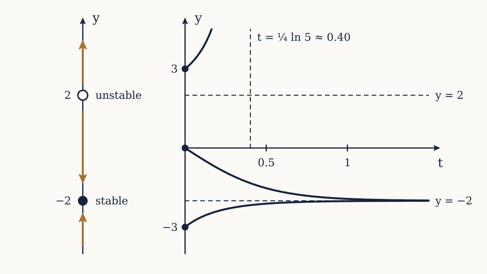
Collapse the picture. Draw the $y$ axis alone, mark the roots of $f$, and on each interval between them put an arrow pointing up where $f>0$ and down where $f<0$. That is the phase line, and it contains everything about the long-run behaviour.

The roots are the equilibria, also called critical points or fixed points: if $f(y^{*})=0$ then the constant function $y\equiv y^{*}$ is a solution, and the system placed exactly there never moves. Every other solution moves along the arrow it starts on and either approaches the equilibrium at the far end or leaves towards infinity. It cannot pass an equilibrium, because that would require two solutions to cross at a point, which uniqueness forbids.

Three kinds of equilibrium exist. An equilibrium with arrows pointing towards it from both sides is stable, or a sink: small disturbances die. With arrows pointing away on both sides it is unstable, or a source: any disturbance grows. With one arrow in and one out it is semi-stable, attracting from one side and repelling on the other.

For the logistic equation $P^{\prime }=rP(1-P/K)$ the roots are $P=0$ and $P=K$. Between them $f>0$ and above $K$ it is negative, so $0$ is unstable and $K$ is stable. That is the S-curve of the earlier lesson, read off in two lines instead of derived by partial fractions, and it also says what the formula did not make obvious: a population starting above $K$ falls to it, and no population ever crosses $K$.

Example. Sketch the phase line for $y^{\prime }=y^2-4$ and describe the fate of solutions starting at $y=-3$, $y=0$ and $y=3$.

The roots are $y=\pm 2$. For $y<-2$, $f=y^2-4>0$, so the arrow points up. For $-2<y<2$ it is negative, arrow down. For $y>2$ it is positive again, arrow up. So $y=-2$ has arrows pointing in from both sides and is stable, while $y=2$ has arrows pointing away and is unstable. A solution from $y=-3$ rises to $-2$. One from $y=0$ falls to $-2$. One from $y=3$ increases without bound, and in fact blows up in finite time, since the growth is quadratic.

Now you. Do the same for $y^{\prime }=y^3-y$, classifying each of the three equilibria.

The linearisation test

Reading signs off a graph is reliable but slow, and there is a one-line test. Put $u=y-y^{*}$, the displacement from an equilibrium, and expand $f$ in a Taylor series about $y^{*}$. Since $f(y^{*})=0$,

For small $u$ the first term dominates, so $u^{\prime }\approx f^{\prime }(y^{*})u$, whose solution is $u=u_0{e}^{f^{\prime }(y^{*})t}$. The conclusion writes itself. If $f^{\prime }(y^{*})<0$ the disturbance decays and the equilibrium is stable. If $f^{\prime }(y^{*})>0$ it grows and the equilibrium is unstable. If $f^{\prime }(y^{*})=0$ the linear term is absent and the test says nothing: $y^{\prime }=y^2$ has a semi-stable equilibrium at zero, $y^{\prime }=-y^3$ a stable one, $y^{\prime }=y^3$ an unstable one, and all three have $f^{\prime }=0$ there.

The number $f^{\prime }(y^{*})$ is more than a sign. Its reciprocal is the time constant of the approach: near a stable equilibrium the gap closes by a factor of $e$ every $1/|f^{\prime }(y^{*})|$ units of time. For the logistic near $P=K$, $f^{\prime }(P)=r-2rP/K$, so $f^{\prime }(K)=-r$ and a population settles towards its capacity with time constant $1/r$, whatever the capacity is. With $r=0.03$ per year that is $33$ years to close $63$ per cent of the gap and $\ln (10)/0.03=77$ years to close $90$ per cent of it. Recovery is slow in a way the carrying capacity alone never tells you.

Terminal velocity read off the equation

A body falling with quadratic drag obeys $v^{\prime }=g-\frac{b}{m}{v}^2$, autonomous and nonlinear. The equilibrium is where drag balances weight, $v_T=\sqrt{mg/b}$, and it is stable because $f^{\prime }(v)=-2(b/m)v$ is negative there. No solving is needed to know that every skydiver approaches the same speed regardless of how they left the aircraft.

Example. A skydiver in a spread posture has $m/b=300$ m. Find the terminal speed and the time constant of the approach to it.

The terminal speed is $\sqrt{300\times 9.81}=54.2$ m s⁻¹. The derivative there is $f^{\prime }(v_T)=-2v_T/300=-0.362$ s⁻¹, so the time constant is $1/0.362=2.8$ s. A useful way to remember it is $v_T/2g$, which is the time gravity alone would take to reach half the terminal speed. The time constant describes the final approach rather than the whole fall: the exact solution from rest is $v=v_T\tanh (gt/v_T)$, which reaches $95$ per cent of terminal after $10.1$ s and about $350$ m, longer than three linearised time constants because early on the drag is far from balancing the weight.

Now you. In a head-down posture the same diver has $m/b=800$ m. Find the terminal speed and the time constant.

A landscape picture

Since $f$ depends on $y$ alone, define $V(y)=-\int f(y)dy$, so that $y^{\prime }=-V^{\prime }(y)$. Then along any solution

so $V$ never increases. The system slides downhill on the graph of $V$ and stops at the bottom of a valley. Stable equilibria are the minima of $V$, unstable ones the maxima, and the depth of a valley says nothing about the rate: the curvature $V^{\prime \prime }(y^{*})=-f^{\prime }(y^{*})$ does. This is the one dimensional case of the potential energy picture in mechanics, and it makes stability visual: a marble in a bowl returns, a marble on a dome does not.

A fishery that collapses without warning

Now put the theory to work on a model that is deliberately simple and still says something. Harvest a logistic population at a constant rate $H$, meaning a fixed catch per year rather than a fixed effort:

The equilibria solve a quadratic, and

Take $r=0.4$ per year and $K=1000$ tonnes. With $H=80$ tonnes per year the square root is $\sqrt{0.2}=0.447$, giving equilibria at $724$ and $276$ tonnes. The upper one is stable, since $f^{\prime }=r-2rP/K$ is $-0.179$ there, and the lower is unstable, with $f^{\prime }=+0.179$. So a stock above $276$ tonnes settles at $724$ and is fished indefinitely, and a stock below $276$ is driven to extinction by the harvest. There is a threshold, and it is not at zero.

Raise the catch and the two equilibria move towards each other. At $H=90$ they are at $658$ and $342$. At $H=rK/4=100$ they meet at $P=K/2=500$, and above that the square root is imaginary: there are no equilibria at all, $P^{\prime }<0$ everywhere, and the population goes to zero from any starting size. The maximum sustainable catch is $rK/4$, exactly the peak growth rate found earlier.

Example. With $r=0.4$ per year and $K=1000$ tonnes, a fishery is harvested at $H=90$ tonnes per year and the stock currently stands at $400$ tonnes. What happens, and what would happen at $500$ tonnes?

The equilibria are at $658$ and $342$ tonnes. A stock of $400$ lies between them, where $f>0$, so it grows to $658$ and stays. A stock of $500$ does the same. Both recover, but the margin above the unstable threshold is only $58$ tonnes in the first case, so a bad year could push the stock below $342$, after which the same harvest drives it to zero.

Now you. The same fishery is harvested at $H=96$ tonnes per year. Find the two equilibria, and say what happens to a stock of $400$ tonnes.

Two features of this deserve naming. The first is that the collapse is not gradual. As $H$ rises from $90$ to $100$ the stable stock falls only from $658$ to $500$, a modest decline that looks like a fishery under control, and then at $H=100$ the stable state disappears entirely and the stock crashes. A qualitative change of this kind, where equilibria collide and annihilate as a parameter passes a critical value, is a bifurcation, and this one is the fold, the commonest of them all.

The second is that the safe margin shrinks as the catch rises: the unstable threshold climbs from $276$ to $342$ to $500$ while the stable state falls. A population sitting on a high yield is close to the boundary of its own basin of attraction, so ordinary environmental noise can push it across even before the bifurcation is reached. The Newfoundland cod fishery, closed by moratorium in 1992 after the northern stock fell to about one per cent of its historic biomass, is the standard illustration, and thirty years later the stock has not returned. The model does not explain that collapse, but it does explain why a fishery can look stable and be about to fail, which is more than a formula for $P(t)$ would have told anyone.

What one variable cannot do

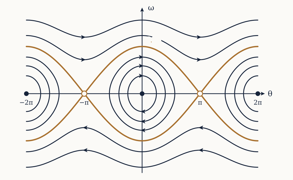
Everything in this lesson rested on solutions being monotone, and that is also the limit. An autonomous first order equation cannot oscillate, cannot overshoot, and cannot return to a state it has left. Yet a plucked string, a swinging pendulum, an RLC circuit and a predator with its prey all do exactly those things.

The escape is to add a second dimension to the state. Position with velocity, or predator with prey, gives a plane to move in, and in a plane a trajectory can circle. Mechanics forces this on us anyway: Newton's second law involves acceleration, so the natural equation is second order. That is where the next lesson starts, and the theory has to be rebuilt for it, because an initial position no longer picks out a single solution.

An initial position no longer determines a trajectory once the equation involves acceleration, and everything built for first order equations has to be redone.

Mechanics forces the change. Newton's second law relates force to the second derivative of position, so the equation for a mass on a spring is $m{x}^{\prime \prime }=-kx$, and knowing where the mass is says nothing about where it goes next: it might be moving either way at any speed. Two numbers are needed, a position and a velocity, and that count is the visible signature of second order.

This lesson builds the structure that makes second order linear equations tractable. It produces no solutions at all, which is deliberate: the structure says how many solutions to look for and what to do once one is found, and the next lesson does the finding.

The operator and its linearity

Write the general second order linear equation in standard form, having divided by the coefficient of $y^{\prime \prime }$:

It is convenient to name the left side. Define $L[y]=y^{\prime \prime }+p{y}^{\prime }+qy$, a rule that takes a twice differentiable function and returns another function. The equation is then $L[y]=g$, homogeneous when $g=0$ and otherwise driven by the forcing $g$.

The one property that matters is that $L$ is linear:

which follows immediately from the derivative of a sum being the sum of derivatives, and from constants passing through derivatives. Everything in this lesson is a consequence of that identity, and nothing in it survives if the equation contains $y^2$ or $\sin y$.

The first consequence is the principle of superposition: if $y_1$ and $y_2$ both solve $L[y]=0$, then so does $c_1{y}_1+c_2{y}_2$ for any constants, since $L$ of that combination is $c_1\cdot 0+c_2\cdot 0$. Solutions of the homogeneous equation can be added and scaled freely, which in the language of the linear algebra course makes them a vector space. The question that then decides everything is what its dimension is.

Existence and uniqueness, and what it buys

The relevant theorem is stronger than Picard's, precisely because linearity removes the possibility of blow-up. If $p$, $q$ and $g$ are continuous on an open interval $I$ containing $t_0$, then for any numbers $y_0$ and $v_0$ there is exactly one solution of $L[y]=g$ on the whole of $I$ with $y(t_0)=y_0$ and $y^{\prime }(t_0)=v_0$.

Three points. The interval is the whole of $I$, not some unknown piece of it. Two numbers are required, matching the order. And uniqueness has an immediately useful corollary: a solution whose value and derivative both vanish at one point is identically zero, because the zero function is one solution with that data and there is only one.

The solution space has dimension exactly two

Take any two solutions $y_1$, $y_2$ of the homogeneous equation, and ask when every solution can be written as $c_1{y}_1+c_2{y}_2$.

Let $y$ be any solution, with $y(t_0)=y_0$ and $y^{\prime }(t_0)=v_0$. We want constants making the combination match those two numbers: