Sign in

Libre University uses your GitHub account. Signing in is only needed to sit a final test, so the score is kept on your profile.

Calculus II

Calculus for quantities that depend on several things at once: partial derivatives, the gradient, optimisation with and without constraints, and integrals over areas and volumes.

Functions of several variables

The pressure of a gas depends on its volume and on its temperature at the same time, and the calculus of one variable, built for a quantity that depends on a single number, has no way to ask how that pressure changes when both are free to move.

The previous course was about y=f(x): one input, one output, a curve with one slope at each point. Almost nothing measured in a laboratory, a factory or a weather station behaves like that. This lesson sets up the objects the rest of this course differentiates and integrates, shows three ways of looking at them, and ends on the precise reason the old machinery breaks. It assumes Calculus I and nothing about vectors or three dimensional geometry.

One output, several inputs

A function of two variables is a rule that takes an ordered pair of real numbers (x,y) and returns one real number, written f(x,y). The pair is best thought of as a single input, a point in the plane, because the question will always be what happens as the point moves. A function of three variables takes a point (x,y,z), and so on.

The ideal gas law is the standard example. For n moles of gas at absolute temperature T in a volume V, the pressure is

p(V,T)=nRTV

with R=8.314 joules per mole per kelvin. One mole at the freezing point of water, T=273.15 K, in a volume of 0.0224 cubic metres, has p=8.314×273.15/0.0224=101383 Pa, which is within a tenth of a percent of the standard atmosphere of 101325 Pa.

Economics has the same shape. In 1928 the mathematician Charles Cobb and the economist Paul Douglas fitted index numbers for American manufacturing from 1899 to 1922, labour L and capital K, to a production function of the form

Q(L,K)=1.01L3/4K1/4

and found that it tracked the actual output index closely for all twenty four years. The exponents add to 1, which has a checkable meaning: doubling both inputs gives 1.01(2L)3/4(2K)1/4=23/4+1/4Q=2Q, so doubling the factory doubles its output.

Weather forecasts supply a third. Since November 2001 the weather services of Canada and the United States have reported a wind chill index computed from the air temperature T in degrees Celsius and the wind speed v in kilometres per hour measured at ten metres:

W(T,v)=13.12+0.6215T-11.37v0.16+0.3965Tv0.16

The output is the temperature which, in near-calm air, would draw heat from exposed skin at the same rate. It is a fitted model of heat loss from a human face, not a law of nature.

Example. Find the wind chill at T=-5 with a wind of v=30.

First 300.16=1.7232. Then the four terms are 13.12, 0.6215×(-5)=-3.1075, -11.37×1.7232=-19.593 and 0.3965×(-5)×1.7232=-3.4163. Their sum is W=-13.0. A thermometer reading of -5 °C in a 30 km/h wind feels like -13 °C.

Now you. Find the wind chill at T=-10 with v=20, to one decimal place.

Answer

Here 200.16=1.6150, and the terms are 13.12, -6.215, -18.362 and -6.403, which sum to W=-17.9. The air is 5 degrees colder than in the example and the wind is lighter, and the second effect recovers only a little of the first.

Where a function is defined

A function of two variables is defined on a set of points in the plane, its domain, and domains in the plane come in far more shapes than intervals on a line.

When a formula is given without comment, the domain is taken to be every point where the formula makes sense. For f(x,y)=9-x2-y2 the square root needs x2+y2≤9, and since x2+y2 is the square of the distance from the origin, the domain is the disc of radius 3 centred there, boundary circle included. For g(x,y)=ln(x-y) the logarithm needs x-y>0, which is every point strictly below the line y=x: a half-plane, with its edge excluded. And h(x,y)=xy/(x2+y2) is defined everywhere except the single point (0,0), a hole of a kind that has no counterpart on the real line, because a point in the plane can be approached from every direction at once. A later lesson shows that this particular hole cannot be filled.

Physical models add restrictions the algebra does not see. The gas law makes sense only for V>0 and T>0, but it is also only accurate where the gas is dilute: squeeze carbon dioxide hard enough at room temperature and it liquefies, while the formula carries on regardless. The wind chill formula is published with the conditions T≤10 and v≥4.8 attached, because outside them the underlying experiment says nothing. The honest domain of a model is where it was tested.

Graphs are surfaces

The graph of y=f(x) needs two axes, one for the input and one for the output. A function of two variables needs three. Its graph is the set of points (x,y,z) with z=f(x,y), drawn with the x and y axes flat on a table and the z axis pointing up, so that above each point of the domain there is exactly one point of the graph, at height f(x,y). Those points form a surface, lying over the domain the way a landscape lies over a map.

Take f(x,y)=x2+y2. The height at each point is its squared distance from the origin, so all points at distance r sit at height r2. The surface is a bowl called a paraboloid, flat at the bottom and steepening outwards. Take instead f(x,y)=9-x2-y2, defined on the disc of radius 3. Squaring z=9-x2-y2 gives x2+y2+z2=9, which says every point of the graph is at distance 3 from the origin in space, and since z≥0 the graph is the upper half of a sphere, a dome sitting on its domain.

The most useful trick for handling a surface is to slice it. Fixing y=b cuts the surface with a vertical plane, and what remains is the curve z=f(x,b), an ordinary function of the single variable x called a trace. The paraboloid sliced at y=2 gives z=x2+4, a parabola lifted by 4. The dome sliced at y=0 gives z=9-x2, a semicircle. Every trace is a problem from the previous course.

The wind chill surface shows how different the traces in two directions can be. Hold the wind at v=30 and the formula collapses to W=-6.473+1.3048T: a straight line, saying that in that wind every degree of real cooling feels like 1.3 degrees. Hold the temperature at -5 instead and W=10.0125-13.3525v0.16, a curve that falls steeply for light winds and flattens for strong ones, since going from 10 to 20 km/h costs 2.3 degrees of wind chill and going from 40 to 50 costs only 0.9. One surface, straight when walked one way and bent when walked the other.

Level curves

The second way of looking at a surface slices it horizontally instead. The level curve of f at height c is the set of points in the domain where f(x,y)=c: cut the surface at height c and drop the cut onto the input plane. Drawing several level curves for equally spaced values of c, each labelled with its value, gives a picture of the whole function using only two dimensions.

For the paraboloid the level curve x2+y2=c is a circle of radius c. At c=1,2,3,4 the radii are 1, 1.414, 1.732 and 2, so the circles crowd together further out. That crowding is the steepening of the bowl: the height rises by the same step between each pair of circles, and it does so over shorter and shorter distances.
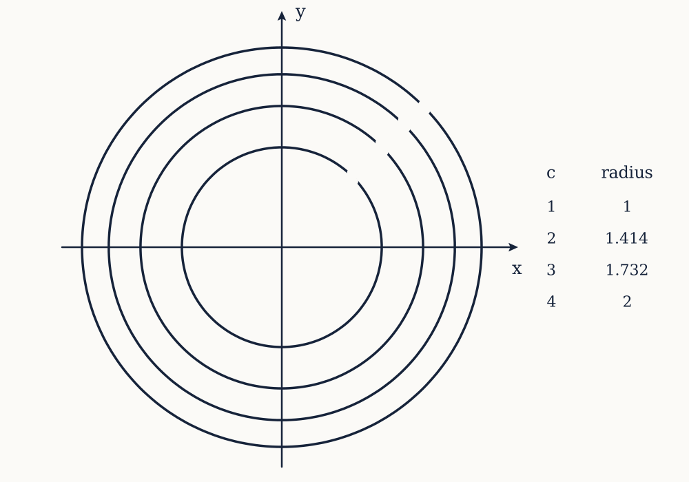
Level curves of x² + y² at c = 1, 2, 3 and 4: circles of radius 1, 1.414, 1.732 and 2. Each step in c is the same, but the circles get closer together further out, where the bowl is steeper.

Level curves have been reinvented in every subject that needed them. Temperature as a function of volume and pressure, T=pV/(nR), has level curves pV=constant, the hyperbolas Robert Boyle measured in 1662 and physicists still call isotherms. Meteorologists draw isobars of equal pressure. Economists draw isoquants, the combinations of labour and capital giving equal output. Cartographers draw contours. The mathematics is the same in every case: a curve along which the function does not change.

For the Cobb-Douglas function the isoquant at output Q0 can be solved explicitly. Write c=Q0/1.01, so that L3/4K1/4=c, and raise both sides to the fourth power to get L3K=c4, that is K=c4/L3. Along an isoquant, capital must rise as the cube of the fall in labour.

Example. A plant with Cobb-Douglas production Q=1.01L3/4K1/4 runs at L=16, K=81. If labour is halved, how much capital keeps output the same?

The current output is 1.01×163/4×811/4=1.01×8×3=24.24, so c=24 and the isoquant is K=244/L3=331776/L3. At L=8 that is 331776/512=648. Halving labour needs eight times the capital, the factor 23 that K=c4/L3 predicts without computing c at all.

Now you. The same plant runs at L=81, K=16. If labour is cut to 27, how much capital keeps output the same?

Answer

Now c=813/4×161/4=27×2=54, and the isoquant is K=544/L3. At L=27 this gives K=8503056/19683=432. Labour fell by a factor of 3, so capital rose by 33=27, from 16 to 432.

Reading a contour map

Contour lines on maps have a mathematical origin. Charles Hutton, reducing the survey of the Scottish mountain Schiehallion made for Nevil Maskelyne's 1774 experiment to weigh the Earth, needed the volume of the mountain and had a mass of spot heights to organise; joining points of equal height turned the numbers into a picture, and his report of 1778 is often credited with the first contours of land relief. A walker's map is a level-curve diagram of height above sea level.

The Ordnance Survey's 1:50,000 Landranger maps of Great Britain draw contours every 10 metres, and at that scale one millimetre on the paper is 50 metres on the ground. Count the contour gaps crossed along a route to get the rise, measure the route on the map to get the run, and divide. Closely packed contours mean a steep slope, widely spaced ones a gentle slope, and walking along a contour means not climbing at all.

Example. On a Landranger map a path crosses five contour gaps in 4 mm of paper. What is its average gradient, and at what angle does it climb?

The rise is 5×10=50 metres and the run is 4×50=200 metres, so the gradient is 50/200=0.25, a slope of one in four. The angle is arctan0.25=14.0 degrees.

Now you. A route crosses eight contour gaps in 5 mm on the same map. Find the gradient and the angle.

Answer

The rise is 80 metres and the run is 250 metres, so the gradient is 0.32 and the angle is arctan0.32=17.7 degrees.

Why one variable is not enough

The contour map already says what goes wrong. On a hillside the steepness depends on which way you walk: straight up the fall line it is greatest, along the contour it is zero, and every compass bearing in between gives something else. A function of one variable has one line through each point to move along; a function of two variables has a slope in every direction.

The paraboloid f(x,y)=x2+y2 at the point (3,4), where f=25, makes this quantitative. Step a distance 0.001 due east, to (3.001,4), and the difference quotient is 6.001. Step due north instead and it is 8.001. Step directly away from the origin, 0.0006 east and 0.0008 north, and it is 10.001. Step along the level circle through the point, 0.0008 west and 0.0006 north, and it is 0.001, heading for zero. Four directions, four limits, 6, 8, 10 and 0, and there are infinitely many more.

The same thing happens with the gas. At T=273.15 K and V=0.0224 cubic metres, warming one mole by a kelvin raises the pressure by 371 Pa, while adding a litre of volume lowers it by 4333 Pa. Doing both at once lowers it by 3977 Pa, close to the sum of the two separate changes, a hint that the separate rates may be enough to recover the rest.

So the derivative of the previous course cannot be reused as it stands. Its difference quotient divided a change in output by a change in input, and here the input change is a step in the plane with both a length and a direction. The limit is affected too: at the hole in xy/(x2+y2) the origin can be approached along infinitely many lines and curves, not just from the left and from the right. And the graph is a surface, so whatever replaces the tangent line must be a plane.

Every one of those needs geometry the previous course never built: distance between points in space, directions described by numbers, and equations for planes. That is the work of the next lesson, which sets up vectors in three dimensions.
Space and vectors

The graph of a function of two variables is a surface in three dimensional space, and nothing in the calculus of one variable says how far apart two points in space are, which way a direction points, or what equation a flat plane has.

The previous lesson met that gap at its end: the slope on a hillside depends on the direction walked, and whatever replaces the tangent line must be a tangent plane. This lesson builds the geometry those ideas need, entirely by computing with coordinates, and assumes only Pythagoras and school trigonometry. Readers who know vectors from Linear Algebra will recognise the dot product; the cross product, and the lines and planes it makes easy, are new.

Coordinates in space

Take three mutually perpendicular number lines meeting at an origin, with the x axis towards you, the y axis to the right and the z axis up, so that, as in the previous lesson, heights are measured along z. A point is an ordered triple (x,y,z). The arrangement is right-handed: curl the fingers of the right hand from the positive x axis to the positive y axis and the thumb points along the positive z axis. Distance does not care about this convention, but the cross product later on does.

Distance comes from Pythagoras applied twice. Between P=(x1,y1,z1) and Q=(x2,y2,z2), the horizontal distance across the floor is (x2-x1)2+(y2-y1)2, and the vertical rise z2-z1 is perpendicular to it, so the two are the legs of a right triangle whose hypotenuse runs from P to Q. Squaring and adding,

|PQ|=(x2-x1)2+(y2-y1)2+(z2-z1)2

From (1,2,3) to (4,6,15) the differences are 3, 4 and 12, and the distance is 169=13. The inside of a standard twenty foot shipping container measures 5.898 by 2.352 by 2.393 metres, so the longest pipe that fits, corner to opposite corner, is 34.786+5.532+5.726=6.786 metres.

The points at distance r from a centre (a,b,c) satisfy (x-a)2+(y-b)2+(z-c)2=r2, the equation of a sphere. Faced with x2+y2+z2-2x+4y-6z=2, complete the square in each variable to get (x-1)2+(y+2)2+(z-3)2=16: radius 4, centre (1,-2,3).

Vectors and components

A point says where; a vector says how far and which way. The displacement from (1,2,3) to (4,6,15) is written ⟨3,4,12⟩, with angle brackets to keep it apart from a point, and the same vector carries (10,10,10) to (13,14,22): a vector has length and direction but no fixed position. The vector from P to Q is head minus tail, ⟨x2-x1,y2-y1,z2-z1⟩. Vectors are printed in bold, 𝐚=⟨a1,a2,a3⟩.

Addition and scaling are componentwise. 𝐚+𝐛 is one displacement followed by the other, which is also how forces combine, and c𝐚 stretches the arrow by the factor c, reversing it when c<0. The length is the distance the arrow covers, |𝐚|=a12+a22+a32, and dividing a non-zero vector by its length gives a unit vector in the same direction: ⟨3,4,12⟩/13=⟨0.2308,0.3077,0.9231⟩. A unit vector is a pure direction, which is how later lessons will say "walk this way".

The unit vectors along the axes are 𝐢=⟨1,0,0⟩, 𝐣=⟨0,1,0⟩ and 𝐤=⟨0,0,1⟩, and every vector combines them: ⟨3,4,12⟩=3𝐢+4𝐣+12𝐤. Engineering texts favour this second notation; the two say the same thing.

The dot product and angles

The dot product multiplies matching components and adds, giving a number:

𝐚⋅𝐛=a1b1+a2b2+a3b3

Its meaning comes from the law of cosines. Put the tails of 𝐚 and 𝐛 together with angle θ between them; the third side of the triangle is 𝐚-𝐛, and the law says |𝐚-𝐛|2=|𝐚|2+|𝐛|2-2|𝐚||𝐛|cosθ. Compute the left side in components instead: each (a1-b1)2 expands to a12-2a1b1+b12, and the three together give |𝐚|2+|𝐛|2-2𝐚⋅𝐛. Comparing,

𝐚⋅𝐛=|𝐚||𝐛|cosθ

So the angle between two non-zero vectors follows from components alone. A positive dot product means an acute angle, a negative one an obtuse angle, and zero means the vectors are perpendicular. That last test is the one used most: ⟨2,-1,3⟩ and ⟨1,5,1⟩ are perpendicular because 2-5+3=0.

Example. A methane molecule has its carbon atom at the centre of a cube and its four hydrogen atoms at alternate corners, which with the carbon at the origin are (1,1,1), (1,-1,-1), (-1,1,-1) and (-1,-1,1). Find the angle between two carbon to hydrogen bonds.

Take 𝐚=⟨1,1,1⟩ and 𝐛=⟨1,-1,-1⟩. The dot product is 1-1-1=-1 and each length is 3, so cosθ=-1/3 and θ=109.47 degrees, the same for every pair by symmetry. Spectroscopy measures the H-C-H angle of methane as 109.5 degrees.

Now you. Find the angle between the long diagonal ⟨1,1,1⟩ of a unit cube and the diagonal ⟨1,1,0⟩ of its floor, to two decimal places.

Answer

The dot product is 2 and the lengths are 3 and 2, so cosθ=2/6=0.8165 and θ=35.26 degrees, the angle at which the long diagonal rises above the floor.

Projection and work

The dot product also splits a vector into a part along a direction and a part across it. If 𝐮 is a unit vector, 𝐛⋅𝐮=|𝐛|cosθ is the length of the shadow 𝐛 casts on the line of 𝐮, called the component of 𝐛 along 𝐮. Multiplying it by 𝐮 gives the projection, and what remains of 𝐛 is perpendicular to 𝐮.

A 20 kg box rests on a ramp rising 3 metres for every 4 of run, so the uphill direction is 𝐮=⟨4,0,3⟩/5. Gravity is 𝐅=⟨0,0,-196.2⟩ newtons, taking g=9.81 metres per second squared, and its component along the ramp is -196.2×3/5=-117.7 newtons, the pull needed to hold the box. The familiar mgsinα has fallen out of the arithmetic without a triangle of forces.

Work is the same computation: a constant force 𝐅 moving an object through a displacement 𝐝 does work W=𝐅⋅𝐝, since only the part of the force along the motion counts. For a 70 kg walker, gravity is ⟨0,0,-686.7⟩ newtons, and over a route with displacement ⟨300,400,120⟩ metres the work is W=-686.7×120, which is 82,404 joules of negative work. The horizontal components are multiplied by zero, which is why the contour map of the previous lesson, counting only height, is enough to reckon the effort of a climb.

The cross product

A plane is fixed by a point and the direction perpendicular to it, so tangent planes will need this: given 𝐚 and 𝐛, find 𝐧=⟨x,y,z⟩ perpendicular to both. That is two equations,

a1x+a2y+a3z=0,b1x+b2y+b3z=0

Multiply the first by b3 and the second by a3 and subtract: z cancels, leaving (a1b3-a3b1)x+(a2b3-a3b2)y=0, which x=a2b3-a3b2 and y=a3b1-a1b3 satisfy. Putting these into the first equation, two terms cancel and z=a1b2-a2b1 remains, and a direct check confirms that all three satisfy both equations. The result is the cross product:

𝐚×𝐛=⟨a2b3-a3b2,a3b1-a1b3,a1b2-a2b1⟩

The indices cycle 1→2→3→1: the first component uses the second and third entries, the second uses the third and first, the third uses the first and second. On the axes, 𝐢×𝐣=𝐤, which is where right-handedness enters: the cross product points along the right thumb when the fingers curl from 𝐚 to 𝐛. Swapping the factors flips every sign, so 𝐛×𝐚=-𝐚×𝐛, and parallel vectors have cross product 𝟎.

The length carries geometry. Expanding both sides in components shows |𝐚×𝐛|2=|𝐚|2|𝐛|2-(𝐚⋅𝐛)2; for ⟨1,2,3⟩ and ⟨4,5,6⟩ the cross product ⟨-3,6,-3⟩ has squared length 54, and 14×77-322=54. Writing the dot product as |𝐚||𝐛|cosθ and using 1-cos2θ=sin2θ,

|𝐚×𝐛|=|𝐚||𝐛|sinθ

which is base times height for the parallelogram with sides 𝐚 and 𝐛. A triangle is half of one: the triangle with corners (1,0,0), (0,2,0) and (0,0,3) has edges ⟨-1,2,0⟩ and ⟨-1,0,3⟩, whose cross product ⟨6,3,2⟩ has length 7, so its area is 3.5.

In mechanics, a force 𝐅 applied at position 𝐫 from a pivot produces the torque τ=𝐫×𝐅, pointing along the axis it tries to turn about, with length equal to the force times its perpendicular lever arm.

Example. A bicycle crank is 175 mm long. With x forward and z up, the pedal is at 𝐫=⟨0.14,0,0.105⟩ metres from the axle, and the rider presses straight down with 𝐅=⟨0,0,-600⟩ newtons. Find the torque.

As a check, |𝐫|=0.0196+0.011025=0.175. The components of 𝐫×𝐅 are 0×(-600)-0.105×0=0, then 0.105×0-0.14×(-600)=84, then 0.14×0-0×0=0. The torque is ⟨0,84,0⟩, of 84 newton metres along the axle. Only the crank's horizontal reach acts as lever arm against a vertical push, and 600×0.14=84 agrees.

Now you. A spanner runs from the bolt to 𝐫=⟨0.2,0.15,0⟩ metres, and a hand pulls its end with 𝐅=⟨0,60,80⟩ newtons. Find the torque and its magnitude, to two decimal places.

Answer

The components are 0.15×80-0×60=12, then 0×0-0.2×80=-16, then 0.2×60-0.15×0=12. So τ=⟨12,-16,12⟩ and |τ|=544=23.32 newton metres, short of the 0.25×100=25 a perpendicular pull would give.

Lines in space

In space a single equation in x, y and z cuts out a surface, so a line needs another description: a motion. Start at P0=(x0,y0,z0) and move in the direction 𝐯=⟨v1,v2,v3⟩; after time t the position is

x=x0+tv1,y=y0+tv2,z=z0+tv3

These parametric equations trace the whole line as t runs over the real numbers. The line through (1,2,3) and (4,6,15) is x=1+3t, y=2+4t, z=3+12t, at the first point when t=0, the second when t=1 and the midpoint (2.5,4,9) when t=12. Another starting point or a rescaled direction describes the same line, worth remembering when two answers look different.

Where a line meets anything is found by substitution. A pole 5 metres tall stands at the origin and sunlight travels in the direction ⟨2,1,-4⟩. The ray through the top is (2t,t,5-4t), which reaches the ground z=0 at t=1.25, the point (2.5,1.25,0). The shadow is 7.8125=2.795 metres long, and the sun stands arctan(5/2.795)=60.8 degrees above the horizon.

Two lines in the plane meet or are parallel; in space they can also be skew. The x axis (t,0,0) and the line (0,s,1) have directions 𝐢 and 𝐣, so they are not parallel, yet one lies at height 0 and the other at height 1 and they never meet, like a road and the railway bridge over it. To test two lines, give them separate parameters, set the coordinates equal, and see whether three equations in two unknowns have a solution.

Planes

A plane is fixed by a point P0=(x0,y0,z0) on it and a normal vector 𝐧=⟨a,b,c⟩ perpendicular to it. A point (x,y,z) lies in the plane exactly when its displacement from P0 is perpendicular to 𝐧, which by the dot product is

a(x-x0)+b(y-y0)+c(z-z0)=0

Collecting constants gives ax+by+cz=d with d=ax0+by0+cz0. So the normal can be read off the coefficients: 2x-y+3z=7 is perpendicular to ⟨2,-1,3⟩, and the floor z=0 has normal 𝐤. The angle between two planes is the angle between their normals. Given three points not on a line instead, the cross product of two edges supplies the normal, the construction tangent planes will use.

Example. A roof has its eaves along the line from (0,0,3) to (8,0,3) and rises to (0,4,6) at the ridge, in metres. Find its equation and its pitch, and the fraction of full sunlight a panel lying on it receives when the direction towards the sun is ⟨-2,-1,4⟩.

The edges from the first point are ⟨8,0,0⟩ and ⟨0,4,3⟩, with cross product ⟨0×3-0×4,0×0-8×3,8×4-0×0⟩=⟨0,-24,32⟩, or ⟨0,-3,4⟩ after dividing by 8, of length 5. The plane is -3y+4z=d, and (0,0,3) gives d=12; the ridge checks, since -12+24=12. The pitch is the angle between this normal and 𝐤: cosθ=4/5, so θ=36.87 degrees. A panel collects sunlight in proportion to the cosine of the angle between its normal and the sun's direction, here (0+3+16)/(521)=0.829, so 83 percent of what it would facing the sun squarely.

Now you. Find the plane through (0,0,3), (6,2,3) and (1,-3,5), and its angle to the horizontal, to one decimal place.

Answer

The edges are ⟨6,2,0⟩ and ⟨1,-3,2⟩, with cross product ⟨4,-12,-20⟩, or ⟨-1,3,5⟩ after dividing by -4. The first point gives d=15, so the plane is -x+3y+5z=15, and the other two points check. Then cosθ=5/35=0.845 and the angle is 32.3 degrees.

The distance from a point Q=(x1,y1,z1) to a plane is a projection. The shortest route runs along the normal, so the distance is the component, along 𝐧, of the displacement from any point of the plane to Q, which works out as |ax1+by1+cz1-d|/|𝐧|. The origin is |0-12|/5=2.4 metres from the roof plane above.

Distance, and what comes next

The formula this lesson began with is the one the next lesson needs first. In the plane the distance from (x,y) to (a,b) is (x-a)2+(y-b)2, and "(x,y) is close to (a,b)" now means that number is small, whatever direction the approach comes from. Limits in several variables are defined that way, and the function xy/(x2+y2) from the previous lesson will show how badly such a limit can behave. The rest of the toolkit is booked: unit vectors name the direction of a directional derivative, the dot product turns a gradient into a slope, and a normal and a point give a tangent plane.

One limit should be stated plainly. Length, distance, the dot product and angles work in any number of dimensions, with extra terms in the same formulas. The cross product does not: in four dimensions the vectors perpendicular to two given ones form a whole plane, so there is no single answer to pick. That is why Linear Algebra, which works in every dimension, does without it, and why this course uses it only in the three dimensional space where graphs of two variable functions live.

Limits and continuity

A point in the plane can be approached from infinitely many directions and along infinitely many curves, so a limit in several variables has far more ways to fail than a limit on the real line, where there are only a left and a right.

The previous lesson ended with the tool this one needs: the distance from (x,y) to (a,b) is (x-a)2+(y-b)2, whatever direction separates them. This lesson uses that number to define limits and continuity in two variables, shows how a limit can depend on the path, and gives a reliable way to prove that one exists. It assumes the one variable limit from Calculus I.

Closeness is distance

In one variable, limx→af(x)=L is a tolerance game: name any tolerance ε on the output, and some tolerance δ on the input keeps f(x) within it. The several variable version keeps the game and changes only how the input tolerance is measured. Instead of |x-a|, use the distance to the point:

lim(x,y)→(a,b)f(x,y)=L

means that for every ε>0 there is a δ>0 such that 0<(x-a)2+(y-b)2<δ forces |f(x,y)-L|<ε.

Geometrically, the points within δ of (a,b) form an open disc, and the condition 0< removes its centre. So the limit is a promise about a punctured disc: every point in it, in every direction, has a value within ε of L. The value at (a,b) itself plays no part and need not exist, as at the hole of xy/(x2+y2).

Producing a δ works the same way as before, with one new habit: bound everything by the distance d. Two facts do most of the work. Each coordinate difference is at most the distance, |x-a|≤d and |y-b|≤d, since a leg of a right triangle is never longer than its hypotenuse. And a dot product is at most the product of lengths, |𝐮⋅𝐯|≤|𝐮||𝐯|, since |cosθ|≤1.

Take lim(x,y)→(0,0)(3x+4y)=0. The quantity 3x+4y is the dot product of ⟨3,4⟩ with ⟨x,y⟩, so |3x+4y|≤5d, and δ=ε/5 works. The bound is sharp: at distance 0.01 in the direction ⟨3,4⟩, the point (0.006,0.008) gives 0.018+0.032=0.05, exactly 5×0.01.

Every path must agree

If the limit is L, then every point of the punctured disc has its value within ε of L, and in particular every point of any path that runs into (a,b). So the values along every path must tend to L: along the x axis, along any line, along a parabola, along a spiral. This gives the standard way to show that a limit does not exist. Find two paths into the point along which the function tends to different values, or one path along which it tends to nothing, and no L can satisfy the definition.

This is the left and right limit test of one variable, with infinitely many sides. It runs in one direction only: agreement along two paths, or ten, or every line, proves nothing, because a path not yet tried may disagree. Paths disprove; they never prove.

A limit that depends on the direction

Take f(x,y)=xyx2+y2, defined everywhere except the origin. Along the x axis, y=0 and the function is 0 at every point, so it tends to 0. Along the y axis it is also 0. Along the diagonal y=x it is x2/2x2=12 at every point, however close to the origin. Two paths, two different values, and the limit does not exist.

All the lines at once tell the whole story. Along y=mx with x≠0,

f(x,mx)=mx2x2+m2x2=m1+m2

which does not depend on x at all: the function is constant along each line through the origin, with the constant set by the slope. The slope m=2 gives 0.4, m=-1 gives -12, and as m runs over the real numbers the constant covers every value from -12 to 12. So every punctured disc around the origin, however small, contains points where f=12 and points where f=-12, and no tolerance smaller than 12 can be met around any candidate L.

Polar coordinates make the same point in one line. Writing x=rcosθ and y=rsinθ, where r is the distance to the origin and θ the angle of the direction, gives f=cosθsinθ=12sin2θ. The distance r has cancelled completely, so the value depends only on the direction. The level curves of f are the lines through the origin, all crowding into the hole with every height from -12 to 12.

Example. Show that x2-y2x2+y2 has no limit at the origin.

Along y=mx the value is x2-m2x2x2+m2x2=1-m21+m2, again constant on each line. The x axis, m=0, gives 1. The line y=x gives 0. The y axis, which is not of the form y=mx and must be checked on its own, has x=0 and value -y2/y2=-1. Three different values along three paths, so there is no limit. In polar coordinates the function is cos2θ-sin2θ=cos2θ, which again has lost r.

Now you. Find the value that 2xyx2+4y2 approaches along the line y=mx, and use it to show that the function has no limit at the origin.

Answer

Along y=mx the value is 2mx2x2+4m2x2=2m1+4m2. The x axis gives 0 and the line y=12x gives 12, so two paths disagree and the limit does not exist.

Every line is not enough

After the examples above it is tempting to check all the lines through the point and, if they agree, declare the limit. The function

g(x,y)=x2yx4+y2

shows why that fails. On the x axis and the y axis it is 0. Along y=mx with m≠0,

g(x,mx)=mx3x4+m2x2=mxx2+m2

and as x→0 the numerator goes to 0 while the denominator goes to m2, so the limit is 0. Every line into the origin gives 0. Numerically, along y=x the values at x=0.1, 0.01 and 0.001 are 0.0990, 0.0100 and 0.0010, heading steadily for zero.

Now approach along the parabola y=x2 instead:

g(x,x2)=x4x4+x4=12

at every point, however close. At (0.01,0.0001) the value is exactly 0.5. So there are points with g=12 in every punctured disc around the origin, and the limit does not exist, even though it is 0 along every straight line. Along y=kx2 the value is k/(1+k2): g is constant on parabolas the way xy/(x2+y2) is constant on lines.

Straight lines are simply the wrong family of paths for this function, and no finite list of families is always the right one. To prove a limit exists, something must control every point of a punctured disc at once.

Polar coordinates and the squeeze

The tool that controls a whole disc is a bound that depends on the distance alone. Suppose that near (a,b)

|f(x,y)-L|≤B(d)

where d is the distance to (a,b) and B(d)→0 as d→0. Given ε, choose δ so that B(d)<ε whenever d<δ, which the one variable limit of B guarantees. Then every point of the punctured disc of radius δ has |f-L|<ε, whatever its direction. This is the squeeze theorem of Calculus I, with f trapped between L-B(d) and L+B(d), and both walls closing in on L as the distance shrinks.

At the origin, polar coordinates are the natural way to find such a bound, because r is the distance. Substitute x=rcosθ, y=rsinθ, simplify, and try to write |f-L| as at most something in r alone. Since |cosθ|≤1 and |sinθ|≤1, any leftover trigonometric factors can be bounded by 1. The one requirement is that the final bound contain no θ: a bound that shrinks for each fixed direction but not uniformly across all of them proves nothing.

Example. Prove that 3x2yx2+y2→0 as (x,y)→(0,0), and find a δ for each ε.

In polar coordinates the numerator is 3r3cos2θsinθ and the denominator is r2, so the function equals 3rcos2θsinθ. Its size is at most 3r, since the trigonometric factors are at most 1. The bound B(r)=3r contains no θ and tends to 0, so the limit is 0, and δ=ε/3 works. As a check, at (0.001,0.001) the function is 0.003×10⁻⁶/(2×10-6)=0.0015, and the bound there is 3×0.001414=0.0042.

Now you. Prove that x2y2x2+y2→0 at the origin, and give a δ that works for ε=0.0001.

Answer

In polar coordinates the function is r2cos2θsin2θ, at most r2 with no θ left, so the limit is 0. Any δ with δ2≤0.0001 works, for instance δ=0.01.

Counting degrees predicts the outcome. In xy/(x2+y2) the numerator and denominator both have degree 2, the powers of r cancel exactly, and a pure function of θ is left, which is what makes the value depend on the direction. In the example the numerator has degree 3, one spare power of r survives, and it drives the whole expression to zero. The rule is a guide, not a theorem, and g=x2y/(x4+y2) misleads it. In polar coordinates

g=rcos2θsinθr2cos4θ+sin2θ

and for each fixed θ with sinθ≠0 this tends to 0 as r→0. But when sinθ is as small as rcos2θ, the denominator shrinks to the size of r2 and the fraction reaches 12; those are the points of the parabola y=x2. No bound in r alone exists, which is exactly the failure the requirement above rules out.

Where continuous functions come from

A function f of two variables is continuous at (a,b) when f(a,b) is defined and lim(x,y)→(a,b)f(x,y)=f(a,b): the limit exists and the function takes the value it predicts. It is continuous on a region when it is continuous at every point of it. Continuity is recognised on sight the same way as in one variable: by building functions from simple ones with operations that preserve it.

The building blocks are the constants and the two coordinate functions x and y. The function x is continuous everywhere because |x-a|≤d, so δ=ε works; likewise y.

Sums, products and quotients follow from the limit laws, and their one variable proofs go through unchanged, because they only ever manipulate output tolerances and never mention how the input distance is measured. The product shows the pattern. If f→L and g→M, write

fg-LM=f(g-M)+M(f-L)

Near the point f stays within 1 of L, so |f|≤|L|+1, and both terms can be made as small as wanted by making |g-M| and |f-L| small, each of which some δ achieves; take the smaller of the two δ values. So products of continuous functions are continuous, and repeating the product and sum rules shows that every polynomial in x and y is continuous everywhere. A quotient is continuous wherever its denominator is not zero, so every rational function is continuous except where the denominator vanishes. That includes xy/(x2+y2) everywhere but the origin, where no value fills the hole.

Composition is the rule that reaches everything else. Suppose u=g(x,y) is continuous at (a,b), and h is a function of one variable continuous at c=g(a,b). Given ε, continuity of h provides an η such that |u-c|<η keeps |h(u)-h(c)|<ε. Continuity of g then provides a δ such that d<δ keeps |g(x,y)-c|<η. Chaining the two, d<δ keeps |h(g(x,y))-h(g(a,b))|<ε. So exy, sin(x2+y), ln(x-y) on the half-plane x>y, and 9-x2-y2 on its disc are all continuous, since each is a continuous function of one variable applied to a polynomial.

The consequence is the same as in Calculus I: most limits are evaluated by substitution. Where nothing divides by zero the limit is the value, so lim(x,y)→(1,2)(x2y+3)/(x+y)=5/3 with no ε in sight. The effort goes into the points where the formula breaks, and composition often handles those too.

Example. What value at the origin makes F(x,y)=sin(x2+y2)x2+y2 continuous there?

Write F=h(u) with u=x2+y2 and h(u)=(sinu)/u. Calculus I gives sinu/u→1 as u→0, so setting h(0)=1 makes h continuous at 0. The polynomial u is continuous with u(0,0)=0, so by the composition rule F tends to h(0)=1, and defining F(0,0)=1 makes it continuous. At (0.1,0.2), where u=0.05, the value is 0.99958.

Now you. What value at the origin makes 1-cos(x2+y2)(x2+y2)2 continuous there?

Answer

With u=x2+y2 the function is (1-cosu)/u2. The Taylor polynomial cosu≈1-12u2 gives the limit 12 as u→0, so the value is 12. At (0.1,0.2) the function is 0.49990.

One variable at a time, and what comes next

A tempting shortcut is to test continuity one variable at a time: freeze y, check the resulting function of x, then freeze x and check the function of y. The function xy/(x2+y2), given the value 0 at the origin, shows that this is not enough. Freeze y=b with b≠0 and the result bx/(x2+b2) is a rational function of x with a denominator that never vanishes, continuous everywhere. Freeze y=0 and the result is the constant 0, also continuous. The same holds with the roles swapped. So the function is continuous in each variable separately at every point, including the origin, and yet it is not continuous at the origin, since along y=x it stays at 12 while its value there is 0.

The explanation is the theme of this lesson. Freezing a variable looks only along the two axes, two paths out of infinitely many, and paths can disprove continuity but never prove it. In three variables nothing changes but the distance formula: a ball replaces the disc.

Where continuity does hold, the next step is to measure slopes, and the idea that failed here as a test of continuity works well as a way of taking them. Freeze every variable but one, and the surface becomes a curve with an ordinary slope that Calculus I can compute. That is the partial derivative, the subject of the next lesson. It inherits the weakness exposed in this section: two slopes along the axes see only two directions, and xy/(x2+y2) will turn up again as a function that has them both at a point where it is not even continuous.

Partial derivatives

A surface has a different slope in every direction through a point, but along the two coordinate directions the slope is an ordinary derivative that the calculus of one variable already knows how to take.

The previous lesson defined limits and continuity in two variables and found that freezing one variable at a time is a poor test of continuity, because it looks along only two paths. As a way of measuring slopes, freezing works well. This lesson defines the partial derivative, computes it with the rules of Calculus I, reads it off real models, differentiates twice, and meets the theorem that makes second derivatives manageable, together with the function where it fails.

Freeze every variable but one

Let f be a function of x and y and fix a point (a,b). Holding y at b leaves x↦f(x,b), a function of one variable, and its ordinary derivative at x=a is the partial derivative of f with respect to x:

fx(a,b)=limh→0f(a+h,b)-f(a,b)h

Only x moves in the quotient; y sits at b throughout. Holding x at a and moving y instead gives fy(a,b), the same limit with f(a,b+k) in place of f(a+h,b).

Two notations are in use and they mean exactly the same thing: fx, compact enough for long calculations, and the Leibniz form ∂f∂x, whose curly ∂ warns that other variables are being held still. Adrien-Marie Legendre used the symbol in 1786 and Carl Jacobi made it standard in 1841.

Take the paraboloid f(x,y)=x2+y2 at (3,4), where f=25. Holding y=4, the difference quotient is

(3+h)2+16-25h=6h+h2h=6+h

which tends to 6, so fx(3,4)=6. The same work in y gives 8+k, so fy(3,4)=8. At h=0.001 the quotients are 6.001 and 8.001, the east and north slopes found by stepping away from (3,4) when this surface first appeared, in the lesson on functions of several variables.

Nobody evaluates that limit for every function. Since fx is an ordinary derivative, every rule of Calculus I applies, and the one new instruction is to treat every other variable as a constant. In x2+y2 the term y2 is a constant as far as x is concerned, so fx=2x and likewise fy=2y, and fx(3,4)=6 falls out by substitution. In x2y3 with y frozen, y3 is a coefficient like the 5 in 5x2, so the x partial is 2xy3 and the y partial is 3x2y2. The product rule returns only when both factors contain the moving variable, and the chain rule whenever the moving variable sits inside another function. In three or more variables nothing changes: gz freezes x and y and differentiates in z.

Example. Find fx and fy for f(x,y)=x2y3+sin(xy), and evaluate both at (1,2).

With y constant, x2y3 gives 2xy3, and sin(xy) needs the chain rule with inner function xy, whose x derivative is y. So fx=2xy3+ycos(xy), and with x constant the same steps give fy=3x2y2+xcos(xy). At (1,2), cos2=-0.4161, so fx=16-0.8323=15.168 and fy=12-0.4161=11.584. A central difference in x with step 0.001 also gives 15.168: a partial derivative can always be checked by nudging one input.

Now you. Find fx and fy for f(x,y)=xexy+y2 at (1,1), to three decimal places.

Answer

In x both factors of xexy move, so the product rule gives fx=exy+xyexy, which at (1,1) is 2e=5.437. In y the factor x is a constant: fy=x2exy+2y=e+2=4.718.

The slope of a slice

Cut the surface z=f(x,y) with the vertical plane y=b and what remains is the curve z=f(x,b), the trace of the surface in that plane. Its slope at x=a is fx(a,b). So fx is the slope of the surface for a walker heading due east, in the direction of increasing x, and fy is the slope for a walker heading due north. Neither says anything about a walker heading north-east.

On the paraboloid, the slice y=4 is the parabola z=x2+16, whose tangent line at x=3 has slope 6. In space that line passes through (3,4,25) and climbs 6 units for each unit east, so it runs along ⟨1,0,6⟩; the slice x=3 gives a tangent line along ⟨0,1,8⟩. Two lines through one point determine a plane, and any tangent plane at (3,4,25) must contain both. Whether the surface actually has one is a question for the next lesson.

Each partial derivative has its own meaning and its own units. The wind chill index W(T,v)=13.12+0.6215T-11.37v0.16+0.3965Tv0.16, with T in degrees Celsius and v in km/h, has WT=0.6215+0.3965v0.16, which at v=30 is 1.305: in that wind each degree of real cooling feels like 1.3 degrees. It also has Wv=0.16v-0.84(-11.37+0.3965T), which at T=-5 and v=30 is -0.123 degrees per km/h. Raising the wind from 30 to 31 km/h lowers the index by 0.121, slightly less than the rate because the curve flattens as the wind grows.

A rate with everything else fixed

In a model, a partial derivative answers the question every controlled experiment asks: change this one thing and hold the rest. The ideal gas law p=nRT/V, with R=8.314 joules per mole per kelvin, has three. With n and V held, nR/V is a constant coefficient; with n and T held, V appears as V-1. So

∂p∂T=nRV,∂p∂V=-nRTV2

and ∂p/∂n=RT/V. For one mole at T=273.15 K in V=0.0224 cubic metres, where p=101383 Pa, these give ∂p/∂T=371.2 Pa per kelvin and ∂p/∂V=-101383/0.0224=-4.526×106 Pa per cubic metre, or -4526 Pa per litre. Finite steps from the same state, taken in the lesson on functions of several variables, found that one extra kelvin raises the pressure by 371 Pa and one extra litre lowers it by 4333 Pa. The temperature figures agree exactly because p is linear in T. The volume step falls short of the rate because p falls less and less steeply as V grows, so a whole litre averages a weakening slope.

Example. A plant has the Cobb-Douglas production function Q=1.01L3/4K1/4, fitted to American manufacturing data in 1928, and runs at L=16, K=81. Find the marginal products QL and QK, the extra output per extra unit of each input with the other held fixed.

Treating K as constant, QL=1.01×34L-1/4K1/4=0.7575(K/L)1/4, and the fourth root of 81/16 is 32, so QL=1.136. Treating L as constant, QK=0.2525(L/K)3/4=0.2525×827=0.0748. An actual extra unit of labour raises output from 24.24 to 25.37, an increase of 1.128, close to the rate. As a check, LQL+KQK=18.18+6.06=24.24=Q. That is no accident: the derivatives show LQL=34Q and KQK=14Q, so if each input were paid its marginal product, labour would take three quarters of the output, close to the share of wages Douglas found in the data.

Now you. Find QL and QK for the same plant at L=81, K=16, to three decimal places.

Answer

Now (K/L)1/4=23, so QL=0.7575×23=0.505, and (L/K)3/4=278, so QK=0.2525×278=0.852. With capital scarce, its marginal product is now the larger. The check 81×0.505+16×0.852=54.54 matches Q.

Second and mixed partials

The partials fx and fy are functions of x and y again, so they have partials of their own. Differentiating fx in x gives fxx, the concavity of the slice y=b, and fyy is the concavity of the slice x=a. The new objects are the mixed partials: fxy differentiates fx with respect to y, measuring how the eastward slope changes as the walker steps north, and fyx differentiates fy with respect to x.

The subscript reads left to right, fxy=(fx)y, while Leibniz notation reads right to left, outwards from f:

fxy=∂∂y(∂f∂x)=∂2f∂y∂x

The conventions are opposite, which matters for the one function below where the order changes the answer. The pure partials are unambiguous: fxx=∂2f∂x2.

For x2+y2, fxx=fyy=2 and fxy=fyx=0: the eastward slope 2x does not depend on y, so walking north does not change it. For x2y3, fxy is the y derivative of 2xy3 and fyx is the x derivative of 3x2y2, and both are 6xy2. Different calculations, same function.

Example. For f(x,y)=x3y2+ye2x, find all four second partial derivatives at (1,2).

The first partials are fx=3x2y2+2ye2x and fy=2x3y+e2x. Then fxx=6xy2+4ye2x, fyy=2x3, and both mixed partials come out as 6x2y+2e2x, one from fx and one from fy. At (1,2), with e2=7.389, fxx=12+59.11=71.11, fyy=2 and fxy=fyx=12+14.78=26.78.

Now you. For f(x,y)=x2siny+xy3, find fxx, fyy and both mixed partials at (2,1), to three decimal places.

Answer

The first partials are fx=2xsiny+y3 and fy=x2cosy+3xy2. Then fxx=2siny=1.683 and fyy=-x2siny+6xy=8.634. Both mixed partials are 2xcosy+3y2=4cos1+3=5.161.

Clairaut's theorem

The agreement of the mixed partials in every example so far is a theorem, used by Leonhard Euler and Alexis Clairaut in the 1730s and 1740s and first proved rigorously by Hermann Schwarz in 1873. If fxy and fyx both exist and are continuous on an open disc around (a,b), then fxy(a,b)=fyx(a,b). Every function built from polynomials, exponentials, sines and logarithms satisfies the hypothesis wherever it is defined, which is why the order of differentiation is normally ignored.

The proof shows where continuity enters. For small h and k, combine the values at the four corners of a small rectangle:

Δ=f(a+h,b+k)-f(a+h,b)-f(a,b+k)+f(a,b)

Read as g(a+h)-g(a) with g(x)=f(x,b+k)-f(x,b), the mean value theorem gives Δ=hg′(c) for some c between a and a+h, and g′(c)=fx(c,b+k)-fx(c,b) is a difference of fx in the y direction, which the mean value theorem again turns into kfxy(c,d). So Δ/hk equals fxy at some point of the rectangle. Grouping the four terms the other way shows it also equals fyx at some point of the rectangle. Shrink the rectangle, and continuity forces both values to their values at (a,b), which must therefore agree.

A check on a less friendly function: for ln(x2+y2), fx=2x/(x2+y2) and fy=2y/(x2+y2), and the quotient rule gives -4xy/(x2+y2)2 for both mixed partials. They are continuous away from the origin, and at (1,2) both equal -8/25=-0.32.

When the mixed partials disagree

The hypothesis of continuity is not decoration. Giuseppe Peano published the standard counterexample in 1884:

f(x,y)=xy(x2-y2)x2+y2,f(0,0)=0

Since |x2-y2|≤x2+y2, its size is at most |xy|, so it is continuous everywhere, and its first partials exist everywhere. The trouble is at the second level.

Since fxy(0,0) is the y derivative of y↦fx(0,y), first find fx all along the y axis. For y≠0, from the definition,

fx(0,y)=limh→0f(h,y)-0h=limh→0y(h2-y2)h2+y2=-y

and at y=0 the quotient is 0 because f(h,0)=0. So fx(0,y)=-y on the whole axis, and fxy(0,0)=-1. Exchanging the roles, fy(x,0)=limk→0x(x2-k2)/(x2+k2)=x, so fyx(0,0)=1. The order of differentiation changes the answer.

Nudges alone confirm it. A central difference with step 10-7 estimates fx(0,0.01)=-0.0100 and fx(0,-0.01)=0.0100, and the outer quotient (-0.01-0.01)/0.02 is -1.0000. Nudging in the other order gives +1.0000, and a smaller outer step changes neither.

Clairaut is not contradicted, because the hypothesis fails. Away from the origin

fxy=(x2-y2)(x4+10x2y2+y4)(x2+y2)3

with numerator and denominator of the same degree, the pattern the previous lesson flagged: in polar coordinates r cancels and only the direction remains. It equals 1 along the x axis, -1 along the y axis and 0 along y=x, however close to the origin, so fxy is not continuous there.

A glimpse of partial differential equations

Once partial derivatives exist, equations can be written between them, and much of physics consists of such equations. In 1822 Joseph Fourier published the heat equation for the temperature u(x,t) at position x along a thin bar at time t:

∂u∂t=α∂2u∂x2

A point warms where the temperature profile curves upwards, where it is colder than the average of its neighbours. The thermal diffusivity α is about 1.11×10⁻⁴ square metres per second for copper.

Checking a proposed solution needs only partial derivatives. For u=e-αk2tsin(kx), holding x gives ut=-αk2u, and holding t gives ux=ke-αk2tcos(kx) and uxx=-k2u. So αuxx=ut everywhere. For a copper bar one metre long with its ends held at zero and a single hump of heat, k=π, and the hump halves when απ2t=ln2, after 0.693/(1.11×10-4×9.870)=633 seconds, about ten and a half minutes.

When a flat plate has reached a steady temperature, ut=0 and the two dimensional heat equation becomes Laplace's equation, uxx+uyy=0, which Pierre-Simon Laplace studied in the 1780s in his work on gravitation. The function x2-y2 satisfies it, since 2-2=0, and so does exsiny. For ln(x2+y2), the first partials above give uxx=2(y2-x2)/(x2+y2)2 and uyy=2(x2-y2)/(x2+y2)2, which cancel. The paraboloid x2+y2 fails, with sum 4: a bowl cannot be a steady temperature, since its centre is colder than everything around it.

Two slopes are not enough

Partial derivatives reduce the calculus of several variables to the calculus of one, but they look along only two lines through each point, and the previous lesson showed how little two lines can see. Its function

g(x,y)=xyx2+y2,g(0,0)=0

takes the constant value m/(1+m2) along each line y=mx through the origin, so it has no limit there and is not continuous. Yet g(x,0)=0 for every x, so the difference quotient (g(h,0)-g(0,0))/h is 0 for every h and gx(0,0)=0. Likewise gy(0,0)=0. Both partial derivatives exist at the origin, and both are zero.

The two slopes describe the plane z=0. Along the diagonal y=x, though, the surface stays at height 12 all the way in, at (0.001,0.001) as much as at (1,1). There is a cliff at the origin that the two coordinate slices step exactly around, and no plane can be tangent to a surface torn like that.

So the existence of fx and fy at a point does not make f smooth there, or even continuous. The partials remain the right numbers to compute, but their existence is too weak to build on. What is needed is a condition that looks in every direction at once: near the point the surface should be close to a plane, with an error small compared with the distance moved. That is differentiability, the existence of a genuine tangent plane, and it is the subject of the next lesson.

Tangent planes and linear approximation

Both partial derivatives of a function can exist at a point where the function is not even continuous, so having partial derivatives cannot be what it means for a function of two variables to be differentiable.

The example is the function whose limit depends on the direction of approach, and it shows that partial derivatives, the one direction slopes of the previous lesson, are too weak on their own. This lesson finds the right notion by asking what a derivative did in one variable and demanding the same of a plane, then turns the resulting tangent plane into approximations and into an estimate of how errors in measured inputs spread into a computed result. It assumes partial derivatives, written fx and fy, and the equation of a plane.

Two slopes are not enough

Take f(x,y)=xyx2+y2 with f(0,0)=0. On the x axis the function is identically 0, so its slope in the x direction at the origin is fx(0,0)=0, and the same argument on the y axis gives fy(0,0)=0. Both partial derivatives exist. Yet along the line y=x the function equals 12 at every point, however close to the origin, so it is not continuous there.

The partials describe a surface along two lines only, the axes through the point. Here the surface is flat along both, at height 0, which suggests that near the origin it should look like the plane z=0. It does not: along the diagonal it stays half a unit above that plane all the way in. Two slopes say nothing about the infinitely many other directions, the same weakness the limit had when only some paths were checked.

Treat the candidate plane as an approximation and measure its error. At (h,h) the function is 12 and the plane is 0, so the error is 12 however small h is. An approximation whose error does not even go to zero is no approximation at all, and that is the property to repair.

What a derivative really promises

In one variable, f′(a) is defined as a limit of slopes, but the same fact can be stated as a promise about approximation. Write the change in f as the tangent line's prediction plus an error:

f(a+h)=f(a)+f′(a)h+E(h)

Dividing by h gives E(h)/h=(f(a+h)-f(a))/h-f′(a), and the definition of the derivative says exactly that this tends to 0. So f is differentiable at a precisely when some number m makes the error of f(a)+mh shrink faster than h itself, E(h)/h→0. The error of a mere continuous function only tends to zero; the error of a differentiable one is small even compared with the step.

This version generalises without any trouble, because it never divides by a vector. A function f of two variables is differentiable at (a,b) if there are numbers A and B such that

f(a+h,b+k)=f(a,b)+Ah+Bk+E(h,k)

with E(h,k)/h2+k2→0 as (h,k)→(0,0). The denominator is the distance from (a,b) to the new point, so the requirement reads: the error of the linear prediction shrinks faster than the distance, in every direction at once.

The numbers A and B are forced. Set k=0 and the condition becomes (f(a+h,b)-f(a,b))/h-A→0, which says A=fx(a,b). Setting h=0 gives B=fy(a,b). So a differentiable function has both partials, and they are the only possible coefficients. Differentiability also forces continuity: as (h,k)→(0,0) the terms Ah, Bk and E all tend to 0, so f(a+h,b+k)→f(a,b).

The pathological function now fails cleanly. Its only candidates are A=B=0, and at (h,h) the error is 12 while the distance is h2, so the ratio is 1/(22h), which grows without bound instead of shrinking. The function is not differentiable at the origin, as its discontinuity already guaranteed.

A well behaved function passes just as cleanly. For f(x,y)=xy at any (a,b), expanding gives (a+h)(b+k)=ab+bh+ak+hk. The partials are fx=b and fy=a, so the error is exactly hk. Since 2|hk|≤h2+k2, the error is at most half the square of the distance d, and |E|/d≤d/2→0. The error is quadratic in the distance, which is the typical pattern.

The tangent plane

When f is differentiable at (a,b), the linear part of the promise, written in terms of x=a+h and y=b+k, is the tangent plane to the graph z=f(x,y):

z=f(a,b)+fx(a,b)(x-a)+fy(a,b)(y-b)

It passes through the point (a,b,f(a,b)) on the surface, and it is the only plane that hugs the surface in the strong sense of the definition: any other plane through that point has an error that shrinks only as fast as the distance, or not at all.

The geometry agrees with the algebra. Slicing the surface with the plane y=b gives a curve whose slope at the point is fx(a,b), so its tangent line runs in the direction ⟨1,0,fx⟩: one step in x, none in y, a rise of fx. The slice x=a gives the direction ⟨0,1,fy⟩. A tangent plane must contain both lines, and the cross product of the two directions is a normal to it:

⟨1,0,fx⟩×⟨0,1,fy⟩=⟨-fx,-fy,1⟩

The plane through (a,b,f(a,b)) with this normal is -fx(x-a)-fy(y-b)+(z-f(a,b))=0, which rearranges to the formula above.

Example. Find the tangent plane to z=9-x2-y2 at the point above (1,2), and compare it with the surface at (1.1,2.1).

The value is f(1,2)=9-1-4=4. The partials are fx=-2x and fy=-2y, so fx(1,2)=-2 and fy(1,2)=-4. The plane is z=4-2(x-1)-4(y-2), which simplifies to z=14-2x-4y, with normal ⟨2,4,1⟩. At (1.1,2.1) the plane gives 14-2.2-8.4=3.4 and the surface gives 9-1.21-4.41=3.38. The error is -0.02, and expanding 9-(1+h)2-(2+k)2 shows that it is exactly -(h2+k2), minus the square of the distance, whatever the step. The plane lies above the surface, as it must for a dome.

Now you. Find the tangent plane to z=xey at the point above (2,0), and use it to estimate the height of the surface at (2.1,0.1).

Answer

Here f(2,0)=2, fx=ey=1 and fy=xey=2 at the point, so the plane is z=2+(x-2)+2y, which simplifies to z=x+2y. At (2.1,0.1) it gives 2.3, against the true value 2.1e0.1=2.3209.

Continuous partials are enough

Checking the definition directly is tedious for anything larger than xy, so in practice differentiability is recognised by a theorem.

Theorem. If fx and fy exist near (a,b) and are continuous at (a,b), then f is differentiable at (a,b).

The idea of the proof is to travel from (a,b) to (a+h,b+k) along two legs parallel to the axes, first to (a+h,b) and then up to (a+h,b+k), so that on each leg only one variable moves and Calculus I applies. By the mean value theorem, the change along the first leg is fx(p)h for some point p on that leg, and the change along the second is fy(q)k for some point q on it. Subtracting the linear prediction leaves

E=[fx(p)-fx(a,b)]h+[fy(q)-fy(a,b)]k

Since |h| and |k| are each at most the distance d, dividing by d gives |E|/d≤|fx(p)-fx(a,b)|+|fy(q)-fy(a,b)|. As the point closes in, p and q are squeezed towards (a,b), and continuity of the partials sends both brackets to 0. That is the definition.

The theorem does its work through the inventory of continuous functions from the lesson on limits and continuity. The partials of a polynomial are polynomials, the partials of exy or sin(x2+y) are built from continuous pieces, and so every function assembled from the usual functions is differentiable wherever its formula and its partials make sense. The pathological function fails the hypothesis, as it must: away from the origin fx=y(y2-x2)/(x2+y2)2, which on the y axis is 1/y and blows up as the origin approaches. The converse of the theorem is false (there are differentiable functions whose partials are not continuous), but they are rarities built to make the point, and the theorem covers everything met in practice.

Linear approximation

Near a point of differentiability, the tangent plane is a cheap substitute for the function. The linear approximation of f at (a,b) is

f(x,y)≈f(a,b)+fx(a,b)(x-a)+fy(a,b)(y-b)

and it needs only three numbers computed once at a convenient point: the value and the two partials. Every estimate nearby is then a matter of multiplying the small changes by the partials and adding.

Example. Estimate 3.022+3.972 from the linear approximation of f(x,y)=x2+y2 at (3,4), and check it against the true value.

At (3,4) the value is 5. The partials are fx=x/x2+y2 and fy=y/x2+y2, which there are 0.6 and 0.8. The steps are h=0.02 and k=-0.03, so the estimate is 5+0.6×0.02+0.8×(-0.03)=5+0.012-0.024=4.988. The true value is 24.8813=4.988116, so the error is about 0.000116, while the distance moved is 0.022+0.032=0.036. The error is a third of a percent of the distance.

Halving both steps, to (3.01,3.985), shows the definition at work. The estimate is 4.994, the error drops to about 0.000029, a quarter of what it was, and the distance halves to 0.018. The ratio of error to distance has halved too, from 0.0032 to 0.0016, and it keeps halving with each halving of the step. That is what shrinking faster than the distance looks like in numbers.

Now you. Use the linear approximation of f(x,y)=xy3 at (9,8) to estimate 9.27.93, and compare with the true value.

Answer

At (9,8) the value is 3×2=6, with fx=y32x=13 and fy=x3y2/3=14. The estimate is 6+13(0.2)+14(-0.1)=6.0417, against the true value 6.0409.

The approximation is only local. Using the same plane to estimate f(4,3), a distance 1.4 away, gives 5+0.6-0.8=4.8, while the true value is again exactly 5. The surface is a cone whose slope turns as the point moves round it, and how far a step can go before the error matters depends on how fast the partials themselves change, which is a question of second derivatives.

The total differential

The linear approximation has a compact notation that is worth adopting because it carries over to any number of variables. For z=f(x,y) the total differential is

dz=fxdx+fydy

where dx and dy are independent small changes in the inputs and dz is the change they produce along the tangent plane. The actual change in z, written Δz, differs from dz by the error term, which is small compared with the size of the step. For three variables, w=f(x,y,z), the definition and the theorem go through word for word with three terms and the distance in space, and dw=fxdx+fydy+fzdz.

Each term answers a separate question: how much does the output move if only this input moves? Near the point, the answers simply add. That additivity is the whole content of differentiability, and it fails for the pathological function, where moving x alone or y alone changes nothing but moving both together changes the value by 12.

For formulas built from products and powers, dividing by the function gives a relative form that is easier to use. The volume of a cylinder is V=πr2h, so

dV=2πrhdr+πr2dh

and dividing through by V=πr2h gives

dVV=2drr+dhh

The relative change in the volume is twice the relative change in the radius plus the relative change in the height. The exponents become weights: a quantity raised to the power n passes on n times its relative change, and a quantity in the denominator passes on its relative change with a minus sign.

Propagating measurement error

Every measured input carries an uncertainty, and a quantity computed from measured inputs inherits one. The total differential says how much. If x is known to within ±Δx and y to within ±Δy, and these are small, then the computed z=f(x,y) is off by at most about

|fx|Δx+|fy|Δy

The absolute values are there because a measurement error can go either way, and the worst case is the one where both terms push in the same direction. This is the standard worst case bound quoted in engineering and in the first year laboratory.

Example. A cylindrical can has a measured radius of 5.0±0.1 cm and height of 12.0±0.1 cm. Estimate the maximum error in its computed volume, absolute and relative.

The volume is V=πr2h=300π, about 942.5 cm³. The differential gives dV=2πrhdr+πr2dh=2π(60)(0.1)+π(25)(0.1)=14.5π, so the volume is uncertain by about 45.6 cm³. The relative form gives the same answer more quickly: 2×0.15+0.112=0.04+0.0083=0.048, a relative error of about 4.8%. As a check, the largest possible can, π(5.1)2(12.1), exceeds 300π by 46.2 cm³, and the smallest, π(4.9)2(11.9), falls short by 44.9 cm³. The differential sits between the two, as a linear estimate of a slightly curved change should.

The breakdown is the useful part. Of the 4.8%, the radius contributes 4% and the height less than 1%, even though both were measured to the same 0.1 cm, because the radius is smaller and is squared. A better volume needs a better calliper for the diameter, not a better ruler for the height.

Now you. One mole of gas at a measured temperature of 300±1 K occupies a measured volume of 0.0250±0.0001 m³. The ideal gas law gives the pressure as P=nRT/V with R=8.314 J/(mol K). Find P and the maximum relative error in it.

Answer

The pressure is P=8.314×300/0.025=99768 Pa, about 99.8 kPa. The differential is dP=nRVdT-nRTV2dV, and dividing by P gives dPP=dTT-dVV. The worst case adds the sizes: 1300+0.00010.025=0.0033+0.0040=0.0073, a relative error of about 0.73%, or roughly 730 Pa.

The worst case bound is deliberately pessimistic. Independent random errors rarely conspire, and statistics replaces the sum of the terms by the square root of the sum of their squares: for the can, 0.042+0.00832=0.041, or 4.1% instead of 4.8%. Either way the differential supplies the terms, and either way the errors must be small enough for the tangent plane to be trusted.

Compositions

Differentiability, a single plane whose error vanishes faster than the distance in every direction at once, is the notion the previous lesson was missing. It implies continuity, it holds wherever the partials are continuous, and its practical form, the total differential, turns small changes in the inputs into a change in the output.

In practice the inputs are rarely free to vary on their own. The temperature recorded by a weather balloon is T(x,y,z) evaluated along the balloon's path, where x, y and z are themselves functions of time. The volume of a can being heated has a radius and height that both depend on the temperature. A formula given in x and y may be needed in terms of the polar r and θ. Each is a composition: a function of several variables whose variables depend on something else.

The total differential already hints at what happens. If z=f(x,y) and both x and y change because time does, then dz=fxdx+fydy should turn into a rate by dividing by dt. Whether that is legitimate, what it becomes when the inner functions have several variables of their own, and how it recovers implicit differentiation in one line are the business of the chain rule, the subject of the next lesson.

The chain rule

A quantity that depends on several variables, each of which is itself changing, changes at a rate that no single partial derivative supplies.

The pressure of a gas depends on its temperature and its volume, and when a gas is heated in a cylinder with a moving piston both change at once. The temperature felt by a weather balloon depends on where the balloon is, and where it is depends on time. The previous lesson ended by noticing that most functions met in practice are compositions of this kind and that its total differential, dz=fxdx+fydy, looks as if it wants to be divided by dt. This lesson proves that it can be, extends the result to inner functions of several variables, and uses it twice: to rewrite partial derivatives in polar coordinates, and to reduce the implicit differentiation of Calculus I to a single formula. It assumes partial derivatives and the definition of differentiability as the existence of a tangent plane whose error shrinks faster than the distance.

The rate along a path

Suppose z=f(x,y), and the point (x,y) moves along a path, so that x=x(t) and y=y(t) are differentiable functions of time. Then z(t)=f(x(t),y(t)) is an ordinary function of one variable, and the question is its derivative. Take f to be differentiable at the point (a,b)=(x(t0),y(t0)), and let time move from t0 to t0+Δt. The inputs move by Δx=x(t0+Δt)-x(t0) and by a similar Δy, and the definition of differentiability says exactly how much z moves:

Δz=fxΔx+fyΔy+E

with both partials evaluated at (a,b) and with an error E satisfying E/d→0, where d=Δx2+Δy2 is the distance the point has moved. Dividing through by Δt gives

ΔzΔt=fxΔxΔt+fyΔyΔt+EΔt

As Δt→0 the first two quotients tend to x′(t0) and y′(t0). The last term is the one to control, and the trick is to route it through the distance: E/Δt=(E/d)(d/Δt). The factor d/|Δt| equals (Δx/Δt)2+(Δy/Δt)2, which tends to the finite speed x′(t0)2+y′(t0)2. The factor E/d tends to 0, because x and y are continuous and so d→0. (When d happens to be 0 the point has not moved and E is 0 as well, so nothing is lost.) A bounded factor times one that vanishes vanishes, and the result is the chain rule along a path:

dzdt=∂z∂xdxdt+∂z∂ydydt

It is the total differential divided by dt, and the derivation is what licenses the division. Each term has a plain meaning: the rate at which z would change if only x were moving, plus the rate if only y were moving. Near a point of differentiability those two contributions simply add, which is the additivity the tangent plane guarantees. With three inputs, as for the weather balloon's T(x,y,z), the same argument gives three terms, one per input.

Differentiability is not a technicality here. Take f(x,y)=x2y/(x2+y2) with f(0,0)=0. It is continuous at the origin, since |f|≤|y|, and it vanishes on both axes, so fx(0,0)=fy(0,0)=0. Along the path x=t, y=t the function equals t/2, so dz/dt=12 at t=0, while the formula would give 0×1+0×1=0. The two partials exist but no tangent plane does, and the chain rule needs the plane.

A gas that heats and expands

The ideal gas law gives the pressure of n moles of gas as P=nRT/V, with R=8.314 J/(mol K). When a piston lets a warming gas expand, temperature pushes the pressure up and volume pulls it down, and the chain rule says which wins.

Example. One mole of gas is at 300 K in a volume of 0.025 m³. It is being heated at 0.5 K per second while the piston withdraws so that the volume grows by 0.0002 m³ per second. Is the pressure rising or falling, and how fast?

The partials of P=RT/V are ∂P/∂T=R/V and ∂P/∂V=-RT/V2. At this state they are 8.314/0.025=332.56 and -8.314×300/0.0252=-3990720, in pascals per kelvin and pascals per cubic metre. The chain rule gives

dPdt=332.56×0.5-3990720×0.0002=166.28-798.14=-631.86

so the pressure, about 99.8 kPa at this moment, is falling at about 632 Pa per second. Heating alone would raise it by 166 Pa each second, but the expansion lowers it by nearly five times as much. As a check, write the state as explicit functions of time, T=300+0.5t and V=0.025+0.0002t, so that P(t)=8.314(300+0.5t)/(0.025+0.0002t). The quotient rule at t=0 gives 8.314(0.5×0.025-300×0.0002)/0.0252=-631.86, the same number by a longer road.

The chain rule is the better road for two reasons. It never needed the formulas for T(t) and V(t), only their rates at the instant, which is what an experiment usually measures. And it splits the answer into contributions that can be read separately, which the single quotient rule computation hides.

Now you. A beetle crosses a metal plate whose temperature is T(x,y)=80-x2-2y2 degrees Celsius, with x and y in metres. At time t seconds it is at x=1+2t, y=3-t. How fast is the temperature it feels changing at t=0?

Answer

At t=0 the beetle is at (1,3), where Tx=-2x=-2 and Ty=-4y=-12. Its velocity is dx/dt=2, dy/dt=-1. The chain rule gives dT/dt=(-2)(2)+(-12)(-1)=-4+12=8, so the temperature it feels is rising at 8 degrees per second: moving in x cools it, but moving towards smaller y warms it more.

Two independent variables

Often the intermediate variables depend on more than one thing. Suppose z=f(x,y) with x=g(s,t) and y=h(s,t), so that z is ultimately a function of s and t. The partial derivative ∂z/∂s holds t fixed, and with t fixed the point (x,y) simply moves along a path parametrised by s. The rule of the first section applies word for word, with s in the role of time and ordinary derivatives replaced by partials:

∂z∂s=∂z∂x∂x∂s+∂z∂y∂y∂s

and the same with t in place of s gives ∂z/∂t. Nothing new had to be proved.

The bookkeeping is easiest to hold as a tree of dependencies. Put z at the top. It depends on x and on y, so two branches lead down from it. Each of x and y depends on s and on t, so two branches lead down from each of them, four in all. To find ∂z/∂s, follow every route from z down to s: there are two, one through x and one through y. Along each route multiply the derivatives on its branches, and add the routes. The same recipe handles any number of layers and variables. With w depending on three intermediate variables that each depend on four independent ones, every partial of w has three terms, one per route.

Take z=x2y with x=s2+t and y=st, at (s,t)=(1,2), where x=3 and y=2. The top level gives zx=2xy=12 and zy=x2=9. The lower level gives xs=2s=2, xt=1, ys=t=2 and yt=s=1. Following the routes, ∂z/∂s=12×2+9×2=42 and ∂z/∂t=12×1+9×1=21. Substituting first gives z=(s2+t)2st, and differentiating that directly at (1,2) produces 42 and 21 again.

One warning about notation. The symbols ∂z/∂x and ∂x/∂s look like fractions that should cancel to ∂z/∂s, and they do not, because each carries a different variable held fixed: the first holds y fixed, the second holds t fixed. The product along one route is only part of the answer, and the other route supplies the rest. In one variable the tree has a single route, which is why the chain rule of Calculus I has a single product and fractions seem to cancel.

Polar coordinates

The most common change of variables in the plane is to polar coordinates, x=rcosθ and y=rsinθ. A function given as f(x,y) becomes a function of r and θ, and its partials in the new variables follow from the tree with s and t renamed. The inner partials are ∂x/∂r=cosθ, ∂y/∂r=sinθ, ∂x/∂θ=-rsinθ and ∂y/∂θ=rcosθ, so

fr=fxcosθ+fysinθ,fθ=-fxrsinθ+fyrcosθ

The first is the rate of change of f as the point moves straight out from the origin at unit speed. The second is the rate per radian as the point swings round a circle of radius r; since a radian of turn covers a distance r, the rate per unit of distance along the circle is fθ/r. A quick sanity check is f=x2+y2, which is r itself. Its partials are x/r=cosθ and y/r=sinθ, and the formulas give fr=cos2θ+sin2θ=1 and fθ=-rcosθsinθ+rsinθcosθ=0, exactly what the derivatives of r with respect to r and θ should be.

Example. For f(x,y)=x2y, find fr and fθ at the point (3,4), and check them by rewriting f in polar form.

The point has r=5, cosθ=0.6 and sinθ=0.8. The Cartesian partials are fx=2xy=24 and fy=x2=9. Since rsinθ=y=4 and rcosθ=x=3, the formulas give fr=24×0.6+9×0.8=14.4+7.2=21.6 and fθ=-24×4+9×3=-96+27=-69. For the check, substitute to get f=r3cos2θsinθ. Then fr=3r2cos2θsinθ=3×25×0.36×0.8=21.6, and the product rule gives fθ=r3(cos3θ-2cosθsin2θ)=125(0.216-0.768)=-69. Both agree.

The two descriptions measure the same steepness in different frames. The sum fx2+fy2=576+81=657 equals fr2+(fθ/r)2=466.56+190.44=657, because the radial and circular directions are perpendicular unit directions just as the x and y directions are, a fact the next lesson explains.

Now you. For f(x,y)=x2-y2, find fr and fθ at the point (4,3), and check them against the polar form f=r2cos2θ.

Answer

Here r=5, cosθ=0.8, sinθ=0.6, fx=2x=8 and fy=-2y=-6. So fr=8×0.8-6×0.6=2.8 and fθ=-8×3+(-6)×4=-48. From the polar form, cos2θ=0.64-0.36=0.28 and sin2θ=2×0.8×0.6=0.96, so fr=2rcos2θ=2.8 and fθ=-2r2sin2θ=-48.

Implicit differentiation in one line

Calculus I found the slope of a curve such as x2+y2=25 by differentiating both sides with y treated as an unknown function of x, then solving for dy/dx. The chain rule explains why that works and compresses it into a formula. Write the curve as F(x,y)=0, and suppose that near some point on it the curve is the graph of a differentiable function y=y(x). Then F(x,y(x))=0 for every x nearby. The left side is a composition of exactly the kind this lesson handles: a path through the plane parametrised by x itself, with dx/dx=1. Its derivative is zero, because it is constantly zero, and the chain rule gives

Fx⋅1+Fydydx=0,sodydx=-FxFy

wherever Fy≠0. For the circle, F=x2+y2-25 gives dy/dx=-2x/2y=-x/y, which at (3,4) is -34, perpendicular to the radius of slope 43 as a tangent to a circle must be.

The argument assumed the curve is a graph near the point. The implicit function theorem, whose proof belongs to analysis, guarantees it: if F has continuous partials and Fy≠0 at a point of the curve, then near that point the curve is the graph of a differentiable function of x. Where Fy=0 but Fx≠0, the roles swap, dx/dy=-Fy/Fx=0, and the tangent is vertical. Where both vanish, the formula says nothing, and the curve may do something other than pass smoothly through.

The same reasoning works one dimension up. A surface F(x,y,z)=0 defines z implicitly as a function of x and y, and holding y fixed turns it into the case just done, so ∂z/∂x=-Fx/Fz and ∂z/∂y=-Fy/Fz wherever Fz≠0.

The folium of Descartes

The curve x3+y3=6xy is the folium, or leaf, of Descartes. He proposed it in 1638 as a challenge to Pierre de Fermat, who had announced a method for finding tangents, and Fermat found them without difficulty. It has a loop in the first quadrant with its tip at (3,3), since 27+27=54=6×9, and two tails running off towards the line x+y=-2.

Example. Verify that (43,83) lies on the folium x3+y3=6xy, and find the slope of the curve there.

On the curve: x3+y3=6427+51227=57627=643, and 6xy=6×329=643. With F=x3+y3-6xy, the partials are Fx=3x2-6y and Fy=3y2-6x, so

dydx=-3x2-6y3y2-6x=2y-x2y2-2x

At the point, 2y-x2=163-169=329 and y2-2x=649-83=409, so the slope is 3240=0.8. The Calculus I route, differentiating x3+y3=6xy term by term to get 3x2+3y2y′=6y+6xy′ and solving for y′, lands on the same expression after two more lines of algebra. The formula skips those lines.

At the tip (3,3) the same expression gives (6-9)/(9-6)=-1, as the symmetry of the curve under swapping x and y demands. The loop has a vertical tangent where Fy=0, that is where y2=2x, and substituting into the curve locates it at (25/3,24/3), about (3.17,2.52). At the origin both Fx and Fy vanish, the formula reads 0/0, and the theorem's hypothesis fails for a visible reason: the curve crosses itself there, passing through twice, once tangent to each axis, so it has two tangents and is not the graph of any single function.

Now you. Check that (2,1) lies on the curve x2+xy+y2=7, find the slope there, and write the tangent line.

Answer

The point gives 4+2+1=7. With F=x2+xy+y2-7, Fx=2x+y=5 and Fy=x+2y=4, so dy/dx=-54=-1.25. The tangent line is y-1=-1.25(x-2), that is y=3.5-1.25x.

Slopes in other directions

The chain rule came straight out of the tangent plane: divide the linear approximation by a small change in the underlying variable and let the error vanish. It gives the rate of change along any path, extends to any tree of dependencies by adding one product per route, converts partial derivatives between coordinate systems, and differentiates curves and surfaces defined implicitly.

Look again at what the ingredients measure. On a hill whose height is z=f(x,y), fx is the slope for a walker heading due east and fy for one heading due north. Polar coordinates added fr, the slope for a walker heading straight away from the origin, but that direction too was chosen by a coordinate system. A walker setting off north east, or on any bearing at all, wants the slope in that direction, and no partial derivative supplies it.

The chain rule already holds the raw material. Walking in a straight line at unit speed is a path, and the rate of change along it depends only on fx, fy and the direction of travel. Turning that into the slope in every direction at once, finding which direction is steepest, and seeing why the pair fx, fy behaves like a vector are the work of the next lesson, on the gradient.

The gradient

Partial derivatives give the slope of a surface only along the two coordinate directions, yet a walker on a hillside can set off on any bearing, and the slope depends on which one.

The previous lesson ended on this gap, and on a hint: the chain rule, which differentiates f(x(t),y(t)) as fxx′(t)+fyy′(t), gives the rate of change along any path, and walking in a straight line at unit speed is a path. This lesson defines the slope in every direction, shows that two numbers contain all of them, and draws out the geometry. It assumes partial derivatives, the chain rule along a path, and the dot product with its formula 𝐚⋅𝐛=|𝐚||𝐛|cosθ.

The slope in any direction

A direction in the plane is a unit vector 𝐮=⟨a,b⟩ with a2+b2=1. Starting at (x0,y0) and walking a distance h in that direction reaches (x0+ha,y0+hb), and the change in height divided by the distance walked is a difference quotient like any other. The directional derivative of f at (x0,y0) in the direction 𝐮 is its limit:

D𝐮f(x0,y0)=limh→0f(x0+ha,y0+hb)-f(x0,y0)h

The insistence on a unit vector is what makes this a slope. With |𝐮|=1 the parameter h is the distance travelled, so the quotient is rise over run. A direction given as ⟨3,4⟩ must first be divided by its length 5, or the answer comes out five times too large.

The partial derivatives are two special cases. Taking 𝐮=𝐢=⟨1,0⟩ gives the quotient (f(x0+h,y0)-f(x0,y0))/h, whose limit is fx, and 𝐮=𝐣 gives fy.

The definition can be applied as it stands. For the paraboloid f(x,y)=x2+y2 at (3,4), in the direction 𝐮=⟨0.6,0.8⟩ pointing away from the origin, the new point is (3+0.6h,4+0.8h) and

f(3+0.6h,4+0.8h)=9+3.6h+0.36h2+16+6.4h+0.64h2=25+10h+h2

The quotient is 10+h, so D𝐮f(3,4)=10. That is the value the first lesson of this course found numerically by stepping 0.001 outward and getting 10.001. But every new direction would need the expansion again.

Two numbers contain every slope

The chain rule removes the labour. Fix the point and the direction, and walk the line through the point at unit speed by setting

g(t)=f(x0+ta,y0+tb)

This is a function of the single variable t, and the difference quotient in the definition is exactly (g(h)-g(0))/h, so D𝐮f(x0,y0)=g′(0). Now g is f evaluated along the path x(t)=x0+ta, y(t)=y0+tb, whose derivatives are the constants x′(t)=a and y′(t)=b. If f is differentiable, the chain rule along a path gives g′(t)=fxa+fyb, and at t=0

D𝐮f(x0,y0)=fx(x0,y0)a+fy(x0,y0)b

The right side is a dot product. The vector of partial derivatives is called the gradient of f and written with the symbol ∇, read "del" or "nabla":

∇f=⟨fx,fy⟩,D𝐮f=∇f⋅𝐮

Two numbers computed once at a point now give the slope in every direction through it. For three variables nothing changes but the length: ∇f=⟨fx,fy,fz⟩, the line is (x0+ta,y0+tb,z0+tc), and the chain rule produces three terms instead of two. On the paraboloid, ∇f=⟨2x,2y⟩=⟨6,8⟩ at (3,4), and ⟨6,8⟩⋅⟨0.6,0.8⟩=3.6+6.4=10, without expanding anything.

The hypothesis matters. Take f(x,y)=x2y/(x2+y2) with f(0,0)=0. Along any line through the origin f(ha,hb)=ha2b, so every directional derivative exists and equals a2b. Both partials are 0 (put b=0, then a=0), so the formula would predict 0 in every direction, yet along ⟨0.6,0.8⟩ the true slope is 0.36×0.8=0.288. This function has a slope in every direction yet no tangent plane, and the formula holds for differentiable functions only, which includes every function whose partials are continuous.

Example. Find the slope of f(x,y)=x3-2xy+y2 at (1,2) in the direction of ⟨3,4⟩.

The partials are fx=3x2-2y and fy=-2x+2y, so at (1,2) they are 3-4=-1 and -2+4=2, and ∇f(1,2)=⟨-1,2⟩. The direction has length 5, so 𝐮=⟨0.6,0.8⟩. Then D𝐮f=-1×0.6+2×0.8=-0.6+1.6=1. A difference quotient with a step of 10-6 gives 1.0000008, agreeing.

Now you. Find the rate of change of f(x,y,z)=xyz at (1,2,3) in the direction of ⟨2,-1,2⟩.

Answer

The gradient is ⟨yz,xz,xy⟩=⟨6,3,2⟩ at the point. The direction has length 3, so 𝐮=13⟨2,-1,2⟩ and D𝐮f=13(12-3+4)=133=4.333.

The direction of steepest increase

The dot product formula turns the directional derivative into geometry. If θ is the angle between ∇f and the unit vector 𝐮, then

D𝐮f=|∇f||𝐮|cosθ=|∇f|cosθ

since |𝐮|=1. Only cosθ depends on the choice of direction, and it lies between -1 and 1. So when ∇f≠𝟎, the slope is greatest at θ=0, walking along the gradient itself, where it equals |∇f|. It is least at θ=π, walking straight against the gradient, where it equals -|∇f|. It is zero at θ=π/2, in the two directions perpendicular to the gradient. The gradient points in the direction of steepest increase, and its length is that steepest rate.

The first lesson of this course found four slopes of the paraboloid at (3,4) by brute force: 6 due east, 8 due north, 10 directly away from the origin, and 0 along the level circle. All four are ⟨6,8⟩⋅𝐮. The third is the largest possible, because ⟨0.6,0.8⟩ is the gradient's own direction and |⟨6,8⟩|=10, and the fourth is zero because ⟨-0.8,0.6⟩ is perpendicular to it. The infinitely many other directions that lesson left open lie between -10 and 10 according to the cosine.

The same picture explains an identity from the previous lesson, where f=x2y at (3,4) had fx2+fy2=657 and also fr2+(fθ/r)2=21.62+13.82=657. The radial unit vector there is 𝐞r=⟨0.6,0.8⟩ and the unit vector round the circle is 𝐞θ=⟨-0.8,0.6⟩, and with ∇f=⟨24,9⟩ the two dot products are 21.6=fr and -13.8=fθ/r. So fx, fy and fr, fθ/r are the components of one vector, the gradient, measured along two different pairs of perpendicular unit directions. Both sums of squares are |∇f|2, and a length does not depend on which perpendicular axes it is measured along.

Example. A hill has height h(x,y)=500-0.0005x2-0.001y2 metres, with x metres east and y metres north of the summit. A walker stands at (300,200). Which way is steepest uphill, how steep is it, and how does it compare with heading straight for the summit?

The height there is 500-45-40=415 metres. The gradient is ⟨-0.001x,-0.002y⟩=⟨-0.3,-0.4⟩, of length 0.5, so the steepest climb heads in the direction ⟨-0.6,-0.8⟩ at a gradient of 0.5, which is arctan0.5=26.6 degrees. The summit lies in the direction ⟨-300,-200⟩, of length 360.56, so 𝐮=⟨-0.8321,-0.5547⟩ and D𝐮h=0.2496+0.2219=0.4715, about 25.2 degrees. The hill is narrower north to south, so the fall line bends towards the y axis and does not aim at the top.

Now you. On the hill h(x,y)=300-0.002x2-0.0005y2, find the steepest slope at (50,400) and its angle, and the slope met by walking due east from there.

Answer

The gradient is ⟨-0.004x,-0.001y⟩=⟨-0.2,-0.4⟩, so the steepest slope is 0.2=0.447, an angle of 24.1 degrees, heading in the direction ⟨-1,-2⟩. Due east is 𝐢, giving hx=-0.2: a descent of 0.2 metres per metre.

A contour map shows the gradient without any formula. With contours every 10 metres, as on the Ordnance Survey's Landranger maps, the height changes by 10 metres between neighbouring contours, and walking straight across them is walking at slope |∇h|. So the spacing on the ground is 10/|∇h|: at the walker's point, 20 metres, which is 0.4 mm of paper at 1:50,000. The first lesson measured a path crossing five contour gaps in 4 mm and called its gradient 0.25. That is |∇h| only if the path crosses the contours squarely; a path slanting across them is taking a directional derivative, and the ground's true steepest slope there is larger.

Perpendicular to the contours

The slope is zero in the directions perpendicular to ∇f, and walking along a contour means not climbing. The two facts are the same fact. Let x(t), y(t) trace the level curve f(x,y)=c through a point, arriving there at t=0 with velocity 𝐯=⟨x′(0),y′(0)⟩≠𝟎. Since f(x(t),y(t))=c for every t, its derivative is zero, and the chain rule says

fxx′(t)+fyy′(t)=0,that is,∇f⋅𝐯=0

So the gradient is perpendicular to the tangent of the level curve through the point. For the paraboloid at (3,4), the level circle has tangent direction ⟨-4,3⟩, and ⟨6,8⟩⋅⟨-4,3⟩=0. On a map the fall line crosses every contour at right angles, which is why streams, running down the negative gradient, cut the contours squarely.

The gradient therefore serves as a normal to the curve, and the tangent line at (x0,y0) is fx(x-x0)+fy(y-y0)=0. Its slope is -fx/fy, the implicit differentiation formula of the previous lesson, now read as a statement about a perpendicular.

Tangent planes to level surfaces

A function of three variables has level surfaces F(x,y,z)=c rather than curves, and the argument applies to every curve on the surface through a point P: its velocity at P satisfies ∇F⋅𝐯=0. So ∇F(P) is perpendicular to every direction in which the surface can be left along itself, which makes it a normal to the tangent plane, and when it is not 𝟎 the plane is

Fx(P)(x-x0)+Fy(P)(y-y0)+Fz(P)(z-z0)=0

A sphere checks it. For x2+y2+z2=9 at (1,2,2), ∇F=⟨2x,2y,2z⟩=⟨2,4,4⟩, parallel to the radius, as geometry demands, and the plane is x+2y+2z=9. A graph is a level surface too: z=f(x,y) is F=f(x,y)-z=0, with ∇F=⟨fx,fy,-1⟩, minus the normal found earlier in this course by a cross product.

Example. Find the tangent plane to the ellipsoid x24+y2+z29=3 at (2,1,3).

The point lies on it, since 1+1+1=3. The gradient is ⟨x2,2y,2z9⟩=⟨1,2,23⟩, or ⟨3,6,2⟩ after multiplying by 3. The plane is 3(x-2)+6(y-1)+2(z-3)=0, which is 3x+6y+2z=18, meeting the z axis at z=9.

Now you. Find the tangent plane to the surface xyz=6 at (1,2,3).

Answer

The gradient is ⟨yz,xz,xy⟩=⟨6,3,2⟩, so the plane is 6(x-1)+3(y-2)+2(z-3)=0, which is 6x+3y+2z=18.

Gradient descent

To find the lowest point of a function too complicated to solve for, walk downhill: from the current point take a small step along -∇f, the steepest way down, and repeat. With a step size η the rule is 𝐱n+1=𝐱n-η∇f(𝐱n). Augustin-Louis Cauchy proposed it in 1847, and machine learning now uses it to fit models with millions of variables.

Take f(x,y)=x2+3y2, whose minimum is 0 at the origin, starting from (3,1) with η=0.1. The gradient is ⟨2x,6y⟩, so each step sends x to x-0.2x=0.8x and y to y-0.6y=0.4y. The iterates are (2.4,0.4), (1.92,0.16) and (1.536,0.064), with values falling from 12 to 6.24, 3.7632 and 2.3716. The first step did not aim at the minimum: -∇f(3,1)=⟨-6,-6⟩ while the origin lies along ⟨-3,-1⟩, the elongated hill again. The steep y direction settles quickly while x shrinks by only a fifth per step.

The step size is a genuine limitation. With η=0.4 the y update becomes y-2.4y=-1.4y, so y runs 1,-1.4,1.96,-2.744 and the values go 12,6.24,11.54,22.59: each step overshoots the valley floor further than it started. Too small a step crawls, too large a step diverges, and the safe range depends on how sharply the function curves.

Where the gradient vanishes

Suppose a differentiable f has a local maximum at a point, and ∇f≠𝟎 there. Walking a short way along ∇f climbs at rate |∇f|>0 and reaches higher values, so the point was not a maximum. Walking against ∇f rules out a minimum the same way. At a local maximum or minimum, then, ∇f=𝟎: every partial derivative is zero and the tangent plane is horizontal. Gradient descent agrees, since its steps stop exactly where the gradient vanishes.

The converse fails. For f(x,y)=x2-y2 the gradient ⟨2x,-2y⟩ vanishes at the origin, yet the surface rises east and west and falls north and south, like a mountain pass. Setting ∇f=𝟎 finds the candidates, and telling summits, hollows and passes apart is the work of the next lesson.

Maxima and minima

Setting the gradient to zero finds every point where a smooth function of two variables could have a maximum or a minimum, but it does not say which of those points are summits, which are hollows and which are neither.

The previous lesson showed that at a local maximum or minimum the gradient ∇f=⟨fx,fy⟩, the vector of partials that points steepest uphill, must be 𝟎. In Calculus I the sign of f′′ sorted the candidates. This lesson builds the two variable version from the second order Taylor polynomial, uses it to fit a line to data, and then finds the largest and smallest values over a whole region. It assumes partial derivatives, the equality of mixed partials, and the chain rule along a path.

Critical points

A function f has a local maximum at (a,b) if f(a,b)≥f(x,y) for every (x,y) in some disc around (a,b), and a local minimum if f(a,b)≤f(x,y) there. The extreme is absolute if the inequality holds over the whole domain in question. At an interior local extreme where f is differentiable both partials vanish, which Calculus I also shows: on the line y=b the function f(x,b) has a local extreme at x=a, so fx(a,b)=0, and likewise fy(a,b)=0.

A critical point is an interior point of the domain where ∇f=𝟎 or where a partial derivative fails to exist. The second clause matters. The cone f(x,y)=x2+y2 is lowest at the origin, but on the x axis it equals |x|, which has no derivative at 0, so fx(0,0) does not exist and no equation ∇f=𝟎 will find the tip.

Finding critical points means solving two equations in two unknowns, rarely linear, so factoring and substitution are the tools. For f(x,y)=x2+y2-2x+6y+14, setting fx=2x-2 and fy=2y+6 to zero gives the single point (1,-3), where f=4. Completing the square shows what it is: f=(x-1)2+(y+3)2+4 is never below 4, so the point is an absolute minimum. Completing a square is the whole idea of the test below.

Not every critical point is an extreme. For f(x,y)=x2-y2 the gradient ⟨2x,-2y⟩ vanishes at the origin, yet the surface rises along the x axis and falls along the y axis. A critical point with higher and lower values in every disc around it is a saddle point, after the shape of a horse's saddle, or of a mountain pass, the lowest point of the ridge and the highest point of the road across it.

The second order Taylor polynomial

Calculus I approximated a function of one variable by its Taylor polynomial of degree two, g(t)≈g(0)+g′(0)t+12g′′(0)t2, with an error that shrinks faster than t2. The two variable version comes from applying it along a line. Fix a step (h,k) and set g(t)=f(a+th,b+tk), the function seen by a point leaving (a,b) in the direction (h,k). The chain rule gives

g′(t)=fxh+fyk

with the partials evaluated at the moving point. Differentiating again, fx is itself a function along the path, with derivative fxxh+fxyk, and fy has derivative fyxh+fyyk. When the second partials are continuous the mixed ones agree, and

g′′(t)=fxxh2+2fxyhk+fyyk2

Putting t=1, with every partial evaluated at (a,b), gives the second order Taylor polynomial:

f(a+h,b+k)≈f(a,b)+fxh+fyk+12(fxxh2+2fxyhk+fyyk2)

The first three terms are the tangent plane and the bracket corrects for curvature. With continuous second partials the error is small compared with h2+k2, the square of the distance moved. For f=excosy at the origin, f=fx=fxx=1, fy=fxy=0 and fyy=-1, so the polynomial is 1+x+12(x2-y2). At (0.1,0.2) it gives 1.085 against the true 1.08314, while the tangent plane alone gives 1.1, nine times further off.

At a critical point the linear terms are zero, and what is left says how the function leaves the point:

f(a+h,b+k)-f(a,b)≈12(Ah2+2Bhk+Ck2)

with A=fxx, B=fxy and C=fyy at (a,b). The bracket is a quadratic form in h and k, and whether the point is a maximum, a minimum or a saddle is a question about its sign in every direction.

The second derivative test

Complete the square, as for the paraboloid above. If A≠0, then

Ah2+2Bhk+Ck2=A[(h+BAk)2+AC-B2A2k2]

as expanding the square confirms. Write D=AC-B2. If D>0, the bracket is a square plus a positive multiple of a square, zero only when k=0 and then h=0, so in every direction the form has the sign of A. If D<0, the bracket is positive for k=0 and negative for h=-Bk/A with k≠0, so the function rises in some directions and falls in others. (If A=0 and D<0, then B≠0 and the form k(2Bh+Ck) also takes both signs.)

That is the second derivative test. At a critical point where the second partials are continuous, let

D=fxxfyy-fxy2

If D>0 and fxx>0 the point is a local minimum; if D>0 and fxx<0 it is a local maximum; if D<0 it is a saddle; and if D=0 the test says nothing. When D>0, fxx and fyy must share a sign, so either may be checked. The four second partials arranged in a square array are called the Hessian, after the German mathematician Otto Hesse, and D is its determinant.

Discarding the Taylor error is safe because of sizes. When D>0 the form is at least a fixed multiple of h2+k2, while the error is eventually smaller than any such multiple, so near the point it cannot overturn the sign. When D<0 the rising and falling directions are fixed lines, and along each the one variable test applies.

Example. Find and classify the critical points of f(x,y)=x3+y3-3xy.

The partials are fx=3x2-3y and fy=3y2-3x. The first vanishes when y=x2, and substituting into the second gives x4=x, so x(x3-1)=0: the critical points are (0,0) and (1,1). The second partials are fxx=6x, fyy=6y and fxy=-3. At the origin D=0×0-9=-9<0, a saddle: along y=-x the function is 3x2, rising, and along y=x it is 2x3-3x2, falling. At (1,1), D=36-9=27>0 with fxx=6>0, a local minimum, f(1,1)=-1. It is not absolute, since f(x,0)=x3 goes to -∞.

Now you. Find and classify the critical points of f(x,y)=2x3+6xy+3y2.

Answer

fx=6x2+6y and fy=6x+6y. The second gives y=-x, and then the first gives 6x2-6x=0, so the points are (0,0) and (1,-1). With fxx=12x, fyy=6 and fxy=6, the origin has D=0-36=-36, a saddle, and (1,-1) has D=72-36=36>0 with fxx=12>0, a local minimum with value -1.

Saddles, and the case the test cannot decide

For x2-y2 at the origin, fxx=2, fyy=-2 and fxy=0, so D=-4 and the test confirms the saddle; the level curve through the pass is the pair of lines y=±x, crossing in an X. A saddle need not announce itself on the axes. The function x2+4xy+y2 has fxx=fyy=2 and curves upward along both axes, yet D=4-16=-12, and along y=-x it equals -2x2. Checking the axes alone is exactly the mistake the test prevents. The monkey saddle x3-3xy2 is a pass with three ways down instead of two, room for two legs and a tail, and at its centre every second partial is zero.

So the monkey saddle has D=0, and D=0 is a genuine gap. Compare x4+y4 with x4-y4. Both have gradient 𝟎 and every second partial 0 at the origin, so both give D=0. Yet the first is never negative, a minimum, while the second is positive along the x axis and negative along the y axis, a saddle; -x4-y4 adds a maximum with the same D. When D=0 the quadratic form vanishes along at least one line, and the higher terms that the Taylor polynomial discarded decide. The remedy is to study the function itself, by factoring it or by following it along lines and curves through the point.

The least squares line

Charles David Keeling began measuring carbon dioxide on Mauna Loa, Hawaii, in 1958, and the record continues. Here are five annual means, rounded to the nearest part per million, with x counting years from 2019:

YearxCO₂ (ppm)
20190412
20201414
20212416
20223419
20234421

No line passes through all five points, so the question is which line y=mx+c fits best. The miss at each point is the residual yi-(mxi+c). Summing residuals lets misses of opposite sign cancel, and summing their sizes gives a function with corners, so the standard choice, published by Adrien-Marie Legendre in 1805, is to minimise the sum of their squares:

S(m,c)=∑i=1n(yi-mxi-c)2

This is a function of the two unknowns m and c, and its minimum is a critical point. The partials are

∂S∂c=-2∑(yi-mxi-c),∂S∂m=-2∑xi(yi-mxi-c)

Setting the first to zero gives y‾=mx‾+c: the best line passes through the point of means. Setting the second to zero and substituting c=y‾-mx‾ gives ∑xi(yi-y‾)=m∑xi(xi-x‾), and since the deviations yi-y‾ and xi-x‾ each sum to zero, xi may be replaced by xi-x‾ on both sides:

m=∑(xi-x‾)(yi-y‾)∑(xi-x‾)2

The test confirms a minimum. The second partials are Smm=2∑xi2, Scc=2n and Smc=2∑xi, so D=4(n∑xi2-(∑xi)2)=4n∑(xi-x‾)2, positive unless every xi is equal, and Scc>0. Since S is a quadratic polynomial, its Taylor polynomial is exact and the minimum is absolute. Statistics derives the same line from a model of random error.

Example. Fit the least squares line to the Mauna Loa data above.

The means are x‾=2 and y‾=2082/5=416.4. The deviations of y are -4.4, -2.4, -0.4, 2.6 and 4.6, so the numerator is 8.8+2.4+0+2.6+9.2=23 and the denominator is 4+1+0+1+4=10. The slope is m=2.3 and the intercept c=416.4-2.3×2=411.8. The residuals are 0.2, -0.1, -0.4, 0.3 and 0, summing to zero as the first equation demands, with minimum sum of squares 0.30. Carbon dioxide rose by about 2.3 ppm a year. The line predicts 423.3 ppm for 2024 and 425.6 for 2025, and the measured means were 424.61 and 427.35: both above the line, because the rise is itself speeding up, which no straight line can capture.

Now you. The Mauna Loa means for 1960, 1970, 1980 and 1990 were 317, 326, 339 and 354 ppm. With x in years since 1960, fit the least squares line, and compare its slope with the recent one.

Answer

x‾=15 and y‾=1336/4=334. The numerator is (-15)(-17)+(-5)(-8)+(5)(5)+(15)(20)=620 and the denominator is 225+25+25+225=500, so m=1.24 and c=334-1.24×15=315.4. The line is y=1.24x+315.4, a rise of 1.24 ppm a year, little more than half the recent 2.3.

Absolute extrema on a closed and bounded region

A largest value over a region need not exist: f(x,y)=x on the open disc x2+y2<1 gets as close to 1 as it likes without reaching it, and on the whole plane it is unbounded. The extreme value theorem in two variables rules out both failures. A continuous function on a set that is closed, containing all its boundary points, and bounded, fitting inside some disc, attains an absolute maximum and an absolute minimum. As in one variable, the proof belongs to analysis.

If the largest value occurs inside the region, it is a local maximum there, so it is at a critical point. Otherwise it is on the boundary. That gives a finite procedure: evaluate f at the critical points inside the region; on each piece of the boundary, write f as a function of one variable and find its extremes on a closed interval, at critical points and endpoints (the corners); then take the largest and smallest values found. No second derivative test is needed, only comparison.

Example. A triangular plate has corners (0,0), (4,0) and (0,4), and its temperature is T(x,y)=x2+y2-2x-4y+20 degrees Celsius. Find the hottest and coldest points.

Inside, Tx=2x-2 and Ty=2y-4 vanish at (1,2), which lies in the triangle since 1+2≤4, and T(1,2)=15. On the bottom edge, T=x2-2x+20 for 0≤x≤4, giving 19 at x=1 and 20 and 28 at the ends. On the left edge, T=y2-4y+20 gives 16 at y=2 and 20 at both ends. On the slanted edge y=4-x, substitution gives T=2x2-6x+20, which is 15.5 at x=1.5, the point (1.5,2.5), and 20 and 28 at the ends. The coldest point is (1,2) at 15 degrees and the hottest is the corner (4,0) at 28 degrees. As a check, T=(x-1)2+(y-2)2+15 is 15 plus the squared distance from (1,2), and (4,0) is the point of the triangle farthest from it.

Now you. Find the absolute maximum and minimum of f(x,y)=xy-x-2y on the rectangle 0≤x≤4, 0≤y≤3.

Answer

Inside, fx=y-1 and fy=x-2 vanish at (2,1), where f=-2 (a saddle, with D=-1). Each edge is linear, so its extremes are at the corners, where f(0,0)=0, f(4,0)=-4, f(0,3)=-6 and f(4,3)=2. The maximum is 2 at (4,3) and the minimum is -6 at (0,3). The interior critical point is neither.

When the inputs are constrained

Setting ∇f=𝟎 finds the candidates, and D=fxxfyy-fxy2 sorts them by the sign of a quadratic form, except in the degenerate case D=0. The same machinery fits a line to data, and comparing interior critical points with the boundary finds the absolute extremes on a closed and bounded region.

Look again at the hottest point of the plate. At (4,0) the gradient is ⟨6,-4⟩, not 𝟎: the temperature would keep rising if the point could leave the triangle, and it cannot. On a boundary the best point need not be critical, and most real problems live entirely on such a boundary. A box must use a fixed area of cardboard, a factory must spend a fixed budget. The inputs are restricted to a curve or surface, and the question is the best point on it.

Take the simplest case: maximise f=xy on the line x+y=10. Substituting y=10-x gives x(10-x), largest at x=5, so the best point is (5,5) with f=25. There the gradient ⟨y,x⟩=⟨5,5⟩ is not zero, but it is parallel to ⟨1,1⟩, which is perpendicular to the line. Substitution worked only because the constraint was easy to solve; on an ellipse or a sphere it is clumsy or impossible. Turning those parallel gradients into a method that never solves the constraint is the work of the next lesson, on Lagrange multipliers.

Lagrange multipliers

A firm maximising output cannot choose any labour and capital it likes, because it has a budget, and the best point on the budget line is almost never a point where the gradient of output vanishes.

The previous lesson found maxima and minima by setting the gradient ∇f to zero and sorting the critical points with the second derivative test. It ended on the catch: real problems restrict the inputs to a curve or a surface (a fixed amount of material, a budget, a plane to stay on), and the best point there can sit on a steep hillside of f. It assumes the gradient and the fact, proved in an earlier lesson, that ∇g is perpendicular to the level curve of g through the point.

Substituting the constraint

The obvious approach is to use the constraint to eliminate a variable. A farmer with 200 metres of fencing encloses a rectangle of sides x and y, so 2x+2y=200, and wants the area xy as large as possible. Solving the constraint gives y=100-x, the area becomes A(x)=100x-x2 on 0≤x≤100, and A′(x)=100-2x=0 at x=50. The best field is a square of 2500 square metres.

It fails quietly as soon as the constraint is less tidy. Take f(x,y)=x2+y2, the squared distance from the origin, on the ellipse x24+y2=1. Substituting y2=1-x24 gives f=1+3x24, whose derivative 3x2 vanishes only at x=0, where f=1. That is the minimum. The maximum, f=4 at (±2,0), is missed entirely: it sits at the ends of the interval -2≤x≤2 on which the substitution is valid, a restriction the formula 1+3x24 does not remember.

Other constraints cannot be solved at all: the closed curve x4+y4+xy=3 needs a quartic solved for y. What is wanted is a method that takes the constraint as a level set g(x,y)=c and never solves it.

Where a contour touches the constraint

Lay the constraint curve g(x,y)=c over the contour map of f and walk along it. Where the constraint cuts a contour at an angle, f is higher on one side of the crossing and lower on the other, so that point is neither a maximum nor a minimum along the walk. The only places the walk can turn round in f are where the constraint does not cut the contour but grazes it: at a constrained extremum the level curve of f is tangent to the constraint curve.

The chain rule makes this exact. Let 𝐫(t)=(x(t),y(t)) trace the constraint curve, passing the point P at t=0 with velocity 𝐯≠𝟎. If f restricted to the curve is extreme at P, the single variable function f(𝐫(t)) is extreme at t=0, so its derivative vanishes, and by the chain rule along a path

∇f(P)⋅𝐯=0

So ∇f is perpendicular to the constraint at P. So is ∇g, since g(𝐫(t))=c for every t and differentiating gives ∇g(P)⋅𝐯=0. In the plane, two vectors perpendicular to the same nonzero direction lie on one line. Provided ∇g(P)≠𝟎, there is therefore a number λ with

∇f(P)=λ∇g(P)

This is the tangency of the picture restated: the gradients are the normals of the two curves, and parallel normals mean the curves share a tangent line. The number λ, the Greek letter lambda, is called a Lagrange multiplier, after Joseph-Louis Lagrange, who used it in his Mécanique analytique of 1788 for mechanical systems held by constraints. It can be positive, negative or zero.

On a constraint surface g(x,y,z)=c the same argument applies to every curve through P, so ∇f(P) is perpendicular to the whole tangent plane, as is its normal ∇g(P). Again ∇f=λ∇g.

The method

Written out in components, ∇f=λ∇g together with the constraint is a system of equations:

fx=λgx,fy=λgy,g(x,y)=c

That is three equations in the three unknowns x, y and λ, or four in four with z. Solve it, evaluate f at every solution, and compare. The solutions are candidates, like the critical points of the previous lesson, not answers. When the constraint set is closed and bounded, such as an ellipse or a sphere, a continuous f is guaranteed a largest and a smallest value on it, and they are among the candidates (together with any points where ∇g=𝟎, which the argument above excluded). When the set is unbounded, a separate argument is needed that an extremum exists at all.

The ellipse that defeated substitution shows the method at work. With f=x2+y2 and g=x24+y2=1, the equations are 2x=λx2 and 2y=2λy. The first says x=0 or λ=4; the second says y=0 or λ=1. Taking x=0, the constraint gives y=±1 and f=1. Taking λ=4, the second equation forces y=0, so x=±2 and f=4. Both the minimum and the missed maximum appear, and at each the ellipse touches a circle centred on the origin, the level curves of f.

The ellipse x²/4 + y² = 1 with level circles of f = x² + y². It touches the circle f = 1 at (0, ±1), the minimum, and the circle f = 4 at (±2, 0), the maximum, while the dashed circle f = 2.25 cuts straight across it. At the touching points the gradients line up: ∇f = ∇g at (0, −1), where λ = 1, and ∇f = 4∇g at (2, 0), where λ = 4.

Example. An open-topped box is to be made from 12 square metres of sheet metal. What dimensions give the largest volume?

With base x by y and height z, maximise V=xyz subject to g=xy+2xz+2yz=12: the base plus four sides. The system is

yz=λ(y+2z),xz=λ(x+2z),xy=λ(2x+2y)

Every quantity is positive, so nothing vanishes. Multiply the first equation by x and the second by y: both left sides become xyz, so λ(xy+2xz)=λ(xy+2yz), which gives xz=yz and x=y. Multiply the third by z and compare with the first times x: λ(xy+2xz)=λ(2xz+2yz), so xy=2yz and x=2z. The box has a square base twice as wide as it is tall. The constraint becomes 4z2+4z2+4z2=12, so z=1 and the box is 2 by 2 by 1 metres, holding 4 cubic metres, with λ=yzy+2z=24=12. The volume is near 0 for a flat tray or a tall narrow tube, so a largest volume exists and this single candidate is it. A random search over 200000 bases found nothing above 3.99999.

Now you. A closed cylindrical can must hold 500 cubic centimetres. Find the radius and height that use the least metal, to two decimal places.

Answer

Minimise A=2πr2+2πrh subject to πr2h=500. The equations are 4πr+2πh=λ⋅2πrh and 2πr=λπr2. The second gives λ=2r, and the first becomes 4πr+2πh=4πh, so h=2r: the height equals the diameter. Then 2πr3=500, so r=4.30 cm and h=8.60 cm, with area 348.73 square centimetres.

The nearest point of a plane

An earlier lesson found the distance from a point to a plane by projecting onto the normal. Lagrange's method finds it with no geometry, together with the nearest point. Minimising the squared distance avoids a square root.

Example. Find the point of the plane 2x+3y+6z=49 closest to the origin.

Minimise f=x2+y2+z2 subject to g=2x+3y+6z=49. The system ⟨2x,2y,2z⟩=λ⟨2,3,6⟩ gives x=λ, y=3λ2, z=3λ. Substituting into the plane, 2λ+9λ2+18λ=49λ2=49, so λ=2 and the point is (2,3,6), at distance 4+9+36=7. The projection formula |ax1+by1+cz1-d|/|𝐧| agrees, giving 49/7=7. The equations made the point a multiple of the normal, the projection argument in other words. The distance grows without bound far out on the plane, so the single candidate is the minimum.

Now you. The roof of the earlier lesson on vectors lay in the plane -3y+4z=12. Find its point nearest the origin, and the distance.

Answer

⟨2x,2y,2z⟩=λ⟨0,-3,4⟩ gives x=0, y=-1.5λ, z=2λ. Then 4.5λ+8λ=12, so λ=0.96 and the point is (0,-1.44,1.92). Its distance is 2.0736+3.6864=5.76=2.4 metres, matching 12/5.

A production budget

The first lesson of this course met the Cobb-Douglas function Q=1.01L3/4K1/4, fitted in 1928 to American manufacturing output from labour L and capital K. A firm running on it has the budget problem this lesson opened with.

Example. Labour costs £3 a unit, capital £1 a unit, and the budget is £400. Maximise output.

The constraint is 3L+K=400. The partials are QL=34⋅QL and QK=14⋅QK, so the system reads 3Q4L=3λ and Q4K=λ. Replacing λ in the first by the second gives 3Q4L=3Q4K, so L=K, and the budget gives 4L=400: L=K=100, output Q=1.01×100=101, and λ=Q4K=0.2525. The spending splits £300 to labour and £100 to capital, in the ratio of the exponents. Stepping L along the budget line by 0.001 finds the same peak.

Now you. Labour now costs £2 a unit, capital £4, and the budget is £800. Find L, K, the maximum output and λ, to two decimal places.

Answer

The equations 3Q4L=2λ and Q4K=4λ give 3Q8L=Q16K, so L=6K. Then 12K+4K=800 gives K=50 and L=300 (again 600 to labour, 200 to capital). Output is 1.01×3003/4×501/4=193.60, and λ=Q16K=0.24.

What the multiplier measures

Let M(c) be the optimal value when the constraint is g=c, attained at a point (x(c),y(c)) that moves smoothly with c. By the chain rule and then ∇f=λ∇g,

M′(c)=fxx′+fyy′=λ(gxx′+gyy′)=λddcg(x(c),y(c))=λ

because g(x(c),y(c))=c. So λ is the rate at which the best achievable value changes as the constraint is loosened. Economists call it a shadow price: for the firm, λ=0.2525 units of output per extra pound, the most an extra pound of budget is worth. Moving the budget to £401 gives L=K=100.25 and Q=101.2525, up by exactly 0.2525. It is exact here because the exponents add to 1, so output grows in proportion to the budget.

The box shows the approximation. There λ=12, predicting 0.05 more cubic metres for 0.1 more square metres of metal. Redoing the solution with 12.1 square metres gives z=12.1/12 and V=4z3=4.0501, a rise of 0.0501.

When the method misleads

The equations are necessary conditions, and a solution need not be an extremum. On the curve y=x3, written g=y-x3=0, take f=y. Then ⟨0,1⟩=λ⟨-3x2,1⟩ gives λ=1 and x=0, the candidate (0,0). But along the curve f=x3, which passes through 0 without turning: the level line y=0 is tangent to the curve and crosses it anyway.

The other failure is where ∇g=𝟎, which the derivation had to exclude. Minimise f=x on the cusp y2=x3, so g=y2-x3. Every point of the curve has x≥0, so the minimum is 0 at the origin. The system asks 1=-3λx2 and 0=2λy; the first forces λ≠0, then y=0 and x=0, and then 1=0. The system has no solution at all, because at the cusp ∇g=⟨0,0⟩. The honest recipe therefore solves the system, adds the points where ∇g=𝟎, and on unbounded constraints checks what happens far out.

Two constraints at once

In space, two constraints g=c and h=d usually meet in a curve. Its tangent at P is perpendicular to both ∇g and ∇h, and at a constrained extremum ∇f is perpendicular to it too. The vectors perpendicular to a line in space form a plane, and when ∇g and ∇h are not parallel they span it, so

∇f=λ∇g+μ∇h

with a second multiplier μ (mu): five unknowns, matched by three component equations and two constraints.

The plane h=x+y+z=1 cuts the cylinder g=x2+y2=2 in an ellipse. For its highest and lowest points, f=z and ⟨0,0,1⟩=λ⟨2x,2y,0⟩+μ⟨1,1,1⟩. The third component gives μ=1, the first two 2λx=2λy=-1, so x=y, and the cylinder gives x=y=±1. The ellipse peaks at (-1,-1,3) and bottoms out at (1,1,-1).

With that, differentiation in several variables is complete: slopes in every direction, tangent planes, chains of dependence, and extrema with and without constraints. The other half of calculus remains. In one variable the integral followed the derivative as a limit of sums, and a function of two variables asks for the same summing over a region of the plane, the volume under a surface. The next lesson builds it.

Double integrals

A surface z=f(x,y) standing over a region of the plane encloses a volume, and nothing in the calculus of one variable says what that volume is or how to compute it.

The previous lesson finished the differential half of the subject: partial derivatives, gradients, tangent planes and extrema, with and without constraints. The other half of calculus is summing. In one variable the integral ∫abf(x)dx was defined as the limit of sums of thin rectangles, height times width, as the widths shrink to zero, and the Fundamental Theorem then evaluated it with an antiderivative. This lesson builds the two variable integral the same way, from sums of thin boxes, and then shows that it can be evaluated with nothing more than two single integrals, one inside the other. It assumes the single integral with its substitution rule, and the partial derivative's habit of holding one variable fixed while the other moves.

Volume as a limit of sums

Take a function f(x,y) on the rectangle R where a≤x≤b and c≤y≤d, written R=[a,b]×[c,d], and suppose for the moment that f is positive. Cut [a,b] into m equal pieces of width Δx and [c,d] into n pieces of width Δy. The grid lines divide R into mn small rectangles, each of area ΔA=ΔxΔy. Over the small rectangle Rij pick a sample point (xij*,yij*) and erect a box of that base and height f(xij*,yij*). The boxes together approximate the solid under the surface, and their total volume is the double Riemann sum

Smn=∑i=1m∑j=1nf(xij*,yij*)ΔA

The double integral of f over R is the limit of these sums as the grid is refined in both directions, provided the limit exists and is the same for every choice of sample points:

∬RfdA=limm,n→∞∑i=1m∑j=1nf(xij*,yij*)ΔA

When f≥0 this is the volume under the surface and above R. When f takes both signs, the boxes below the plane count negatively, exactly as area below the axis did in one variable. As there, every continuous function on a closed rectangle has a double integral; the proof uses the same uniform continuity argument and is not repeated here.

Take the paraboloid f(x,y)=16-x2-2y2 over the square [0,2]×[0,2], and use an n by n grid. Two sample points are natural. The upper right corner of each small square gives the lowest value of f on it, because f falls as x and y grow, so that sum underestimates. The centre of each square gives the midpoint sum. A few lines of code produce these:

GridRectanglesCorner sumMidpoint sum
2×2434.00049.000
4×41641.50048.250
8×86444.87548.0625
16×1625646.46948.0156
100×10010,00047.75948.0004
1000×10001,000,00047.97648.000004

Both columns close on 48. The corner sums creep up slowly, their error falling roughly like 1n, and even a million boxes leave them wrong in the second decimal place. The midpoint sums miss by exactly 4n2, so doubling the grid quarters the error. What the table cannot do is prove the answer is 48, and a million evaluations for three figures is poor value. The next section finds the exact value with two ordinary antiderivatives.

Slicing: the iterated integral

Freeze x at some value between 0 and 2 and cut the solid with the vertical plane at that x. The cut face is the region under the curve y↦16-x2-2y2 for 0≤y≤2, an ordinary area under a curve, with x acting as a constant. Its area is

A(x)=∫02(16-x2-2y2)dy=[16y-x2y-2y33]02=32-2x2-163

This is partial integration, the reverse of the partial derivative: integrate in y as if x were a number. The result is a function of x alone.

Now stack the slices. A slab of thickness Δx at position x has volume close to A(x)Δx, and adding the slabs and letting Δx shrink is a single integral:

∫02A(x)dx=∫02(803-2x2)dx=1603-163=48

The table's 48 is exact. The integral just computed is written with both steps visible,

∫02∫02(16-x2-2y2)dydx

and called an iterated integral. It is read from the inside out: the inner integral and the inner differential dy belong together, so y runs from 0 to 2 first, and the outer pair, dx with its limits, is done last. Slicing the other way, at fixed y, gives ∫02(16-x2-2y2)dx=883-4y2, and then ∫02(883-4y2)dy=1763-323=48 again.

The slicing argument is the method of Bonaventura Cavalieri, who in 1635 compared solids by comparing their cross sections. It is persuasive, but it quietly assumes that the volume defined by boxes and the volume assembled from slices are the same number. That needs a theorem.

Fubini's theorem

The theorem is named after Guido Fubini, who proved a general form of it in 1907. For continuous functions on a rectangle it says:

If f is continuous on R=[a,b]×[c,d], then ∬RfdA=∫ab∫cdf(x,y)dydx=∫cd∫abf(x,y)dxdy

The reason is visible in the Riemann sum. Choose the sample points on a grid, (xi,yj), and add the boxes column by column rather than all at once. The i-th column contributes (∑jf(xi,yj)Δy)Δx, and the bracket is a Riemann sum for the slice area A(xi)=∫cdf(xi,y)dy. Adding the columns then gives a Riemann sum for ∫abA(x)dx. Adding row by row instead gives the other order. A finite sum can be added in any order, so the only work in the proof is showing that both approximations become good at the same time as the grid is refined, and for a continuous function uniform continuity supplies exactly that.

The hypothesis is not decoration. On the square [0,1]×[0,1] take f(x,y)=x2-y2(x2+y2)2, which is continuous everywhere except the corner (0,0), where it blows up. Because ∂∂yyx2+y2=x2-y2(x2+y2)2, the inner integral in y is 11+x2, and then ∫0111+x2dx=arctan1=π4. Swapping the roles of x and y changes the sign of f, so the other order gives -π4. Two orders, two answers, and neither is the double integral, which does not exist: the function is unbounded, and the Riemann sums near the corner can be made as large as desired of either sign.

For continuous functions, the practical content of the theorem is freedom. The order of integration can be chosen to make the antiderivatives easy.

Example. Evaluate ∬RxexydA over R=[0,1]×[0,2].

Integrating first in x needs integration by parts and leaves a function of y with 1y2 terms that is awkward to integrate next. Integrating first in y is immediate, because x is exactly the factor the chain rule produces: ∂∂yexy=xexy. So

∫02xexydy=[exy]y=0y=2=e2x-1

and then

∫01(e2x-1)dx=e2-12-1=e2-32≈2.19453

A midpoint sum on a 1000×1000 grid gives 2.194527, agreeing to six figures.

Now you. Evaluate ∬RyexydA over R=[0,3]×[0,1], to three decimal places. Choose the order first.

Answer

Integrate in x first, since y is the factor ∂∂xexy produces: ∫03yexydx=e3y-1. Then ∫01(e3y-1)dy=e3-13-1=e3-43≈5.362. A midpoint sum on a 1000×1000 grid gives 5.36184.

Regions between two curves

Few regions of interest are rectangles. For a bounded region D, enclose it in a rectangle R and define F to equal f on D and 0 outside it. Then ∬DfdA is defined as ∬RFdA: the boxes outside D contribute nothing. F jumps at the edge of D, so it is not continuous, but when the edge is made of graphs of continuous functions the jump does no harm. The double integral still exists, and a stronger form of Fubini's theorem still turns it into an iterated integral.

Two shapes of region cover most cases. A region of the first type lies between two curves in x: it is described by a≤x≤b and g1(x)≤y≤g2(x). On the vertical line at a fixed x, F is zero except between g1(x) and g2(x), so the inner integral only runs over that stretch:

∬DfdA=∫ab∫g1(x)g2(x)f(x,y)dydx

A region of the second type lies between two curves in y, described by c≤y≤d and h1(y)≤x≤h2(y), and its integral is ∫cd∫h1(y)h2(y)fdxdy. In both, the outer limits are constants and the inner limits may depend on the outer variable, never the other way round, because the outer variable is the one held fixed while the inner one sweeps.

The limits come from a description of the region, which is usually given in words. Take "the region enclosed by the parabola y=x2 and the line y=2x". The curves meet where x2=2x, at x=0 and x=2, so x runs from 0 to 2. Between those values one curve lies above the other throughout, and testing x=1 shows which: the line gives 2, the parabola 1. So the region is 0≤x≤2, x2≤y≤2x. It is also of the second type: solving each curve for x gives x=y2 on the line and x=y on the parabola, and at a height y between 0 and 4 the line is on the left, so y2≤x≤y.

Example. Evaluate ∬DxydA over the region enclosed by y=x2 and y=2x.

As a region of the first type, the inner integral holds x fixed:

∫x22xxydy=x[y22]x22x=2x3-x52

and then ∫02(2x3-x52)dx=8-6412=83. As a check, the second type gives ∫04y⋅12(y-y24)dy=646-25632=83 as well. A midpoint sum with 1000 columns, each cut into 1000 pieces between the curves, gives 2.666669.

Now you. Evaluate ∬DydA over the region enclosed by the parabola x=y2 and the line x=y+2. Which type makes it one integral rather than two?

Answer

The curves meet where y2=y+2, at y=-1 and y=2, and at y=0 the line (x=2) is to the right of the parabola (x=0). So the region is -1≤y≤2, y2≤x≤y+2, of the second type, and ∫-12y(y+2-y2)dy=[y33+y2-y44]-12=83-512=94. As the first type the lower edge changes formula at x=1, from y=-x to y=x-2, forcing two integrals.

Reversing the order

Sometimes the order a problem arrives in cannot be done at all. Consider

∫01∫y1ex2dxdy

The inner integral asks for an antiderivative of ex2, and there is none among the elementary functions: Joseph Liouville's theory of integration in finite terms, developed in the 1830s, proves that no combination of powers, exponentials, logarithms and trigonometric functions differentiates to it.

Reversing the order means reading the region off the limits and describing it the other way. The limits say 0≤y≤1 and y≤x≤1: at each height y, x runs from the diagonal x=y to the vertical line x=1. That is the triangle with corners (0,0), (1,0) and (1,1). Described as a region of the first type, x runs from 0 to 1, and on the vertical line at x the triangle stretches from the bottom edge y=0 up to the diagonal y=x. So

∫01∫y1ex2dxdy=∫01∫0xex2dydx=∫01xex2dx

because ex2 is constant in y and the inner integral just multiplies it by the length x. That factor x is exactly what the substitution u=x2 needs, and

∫01xex2dx=[ex22]01=e-12≈0.859141

The original order can still be computed numerically, since only the antiderivative is missing, not the integral. A midpoint sum in the order given, 2000 values of y and for each one 2000 points from x=y to x=1, gives 0.8591409, against the exact 0.8591409. Fubini's theorem turned an integral that has no formula in one order into a substitution in the other.

Area, average value and mass

Integrating the constant 1 over D builds boxes of height 1, whose volume equals the area of their base, so

area ofD=∬D1dA

For the region between x=y2 and x=y+2 this is ∫-12(y+2-y2)dy=92, the familiar area between two curves recovered as a special case.

The average value of f over D is defined as in one variable, the total divided by the size: f‾=1area ofD∬DfdA. It is the height of the flat-topped solid on the same base with the same volume. For the paraboloid over [0,2]×[0,2] it is 484=12, between the value 16 at the corner (0,0) and 4 at the corner (2,2).

A thin plate whose density ρ(x,y), in kilograms per square metre, varies from point to point has mass by the same summing: a small rectangle near (x,y) has mass about ρ(x,y)ΔA, and in the limit m=∬DρdA. Its average density is the mass divided by the area.

Example. A plate occupies the region between the parabola y=x2 and the line y=1, with lengths in metres and density ρ=1+y kilograms per square metre. Find its area, mass and average density.

The curves meet at x=±1, and the line is on top, so -1≤x≤1, x2≤y≤1. The area is ∫-11(1-x2)dx=43 square metres. For the mass, ∫x21(1+y)dy=32-x2-x42, and ∫-11(32-x2-x42)dx=3-23-15=3215, about 2.1333 kg. The average density is 3215÷43=1.6 kilograms per square metre, above the plain average of 1+y over 0≤y≤1 (which is 1.5) because the plate is wider near the top, where it is denser. A midpoint sum on 1000 columns of 1000 pieces gives 2.13333.

Now you. A plate occupies the region under y=sinx and above the x-axis for 0≤x≤π, with density ρ=y kilograms per square metre. Find the mass to four decimal places, and the average density.

Answer

The inner integral is ∫0sinxydy=sin2x2, and ∫0πsin2x2dx=π4≈0.7854 kg, using sin2x=1-cos2x2. The area is ∫0πsinxdx=2, so the average density is π8≈0.3927 kilograms per square metre.

A disc in the wrong coordinates

Every region so far has had edges that were easy to write as y in terms of x or x in terms of y. The unit disc, x2+y2≤1, is of both types, and in both it is awkward: -1≤x≤1 and -1-x2≤y≤1-x2. Even its area, ∫-1121-x2dx, needs a trigonometric substitution to reach π. For ∬e-(x2+y2)dA over the disc, the inner integral is ∫e-y2dy between square roots, which has no elementary antiderivative, and here reversing the order does not help, since the disc looks the same either way.

The problem is not the function but the grid. Rectangles in x and y are the wrong pieces for a round region; a disc is naturally described by a distance from the centre and an angle. The next lesson cuts the plane along circles and rays instead, works out the area of the small pieces those cuts produce, and with them evaluates this integral and one that single variable calculus could not reach.

Change of variables

A disc described in x and y has curved limits of integration, y=±a2-x2, and the iterated integrals they produce are usually far harder than the question deserves.

The previous lesson built the double integral ∬RfdA as a limit of sums over small rectangles and evaluated it by Fubini's theorem as two single integrals, first over rectangles and then over regions whose limits are functions. It ended on a mismatch: a disc is a rectangle in no Cartesian sense, and its square roots leak into every inner integral. Polar coordinates describe a disc as a rectangle, and this lesson finds the price of switching to them, uses them on an integral that has no elementary antiderivative, and then generalises to any substitution in two variables. It assumes the double integral and iterated integration, and the cross product of two vectors.

Regions that are rectangles in r and θ

Polar coordinates, met in the lesson on the chain rule as a change of variables for derivatives, locate a point by its distance r from the origin and the angle θ its radius makes with the positive x axis:

x=rcosθ,y=rsinθ,r2=x2+y2

Every point other than the origin gets exactly one pair with r>0 and 0≤θ<2π; the origin, r=0 at any angle, is a single point with no area, so an integral does not notice it.

The payoff is in how regions look. The disc x2+y2≤a2 is 0≤r≤a, 0≤θ≤2π: constant limits on both variables, a rectangle in the rθ plane. The annulus between the circles of radius 1 and 3, the shape of a washer, is 1≤r≤3 with θ running all the way round. A sector, the slice of a pizza of radius 15 between the directions θ=0 and θ=π4, is 0≤r≤15, 0≤θ≤π4, and the upper half disc is the same with 0≤θ≤π. In Cartesian coordinates each of these needs square roots, and the annulus needs splitting into four pieces as well.

Polar regions with variable limits work exactly like the general regions of the previous lesson. The circle x2+y2=2x, of radius 1 centred at (1,0), becomes r2=2rcosθ, that is r=2cosθ, so the disc it bounds is 0≤r≤2cosθ for -π2≤θ≤π2. The inner limit depends on the outer variable, and the order of integration is forced: r inside, θ outside.

Rewriting the integrand is the easy half. The hard half is dA: it is tempting to write drdθ, and it is wrong.

The area of a polar rectangle

A grid of lines of constant r and constant θ cuts the plane into polar rectangles: the region r0≤r≤r0+Δr, θ0≤θ≤θ0+Δθ, a curved box bounded by two arcs and two radii. Unlike the squares of a Cartesian grid, they grow with distance from the origin, because a fixed angle sweeps a longer arc at a larger radius.

The exact area comes from the sector. A sector of radius r and angle Δθ is the fraction Δθ2π of a disc of area πr2, so its area is 12r2Δθ. The polar rectangle is the sector of radius r0+Δr with the sector of radius r0 removed, so its area is

ΔA=12((r0+Δr)2-r02)Δθ=(r0+Δr2)ΔrΔθ=r‾ΔrΔθ

where r‾ is the radius midway across the box. No approximation has been made. The box from r=2 to r=2.1 with Δθ=0.1 has area 12(4.41-4)(0.1)=0.0205, and indeed 2.05×0.1×0.1=0.0205. The box is almost a rectangle of width Δr and length r‾Δθ, the arc length, and the factor r‾ is the stretch that turns an angle into a length.

Now repeat the construction of the double integral with this grid. Cut the region into polar rectangles, sample f at the midpoint of each, and add. The sum is

∑f(r‾cosθ‾,r‾sinθ‾)r‾ΔrΔθ

which is exactly a Riemann sum, over a rectangle in the rθ plane, for the function f(rcosθ,rsinθ)r. As the grid refines it converges both to ∬RfdA and to the iterated integral of that function, so

∬Rf(x,y)dA=∫αβ∫abf(rcosθ,rsinθ)rdrdθ

The area element is dA=rdrdθ. The first check is the disc itself: ∫02π∫0ardrdθ=2π⋅a22=πa2. Forgetting the r gives 2πa, the circumference, which is not even measured in the right units.

A disc of varying density

The previous lesson computed the mass of a flat plate as the integral of its surface density, M=∬RρdA. A round plate whose density depends only on the distance from the centre is what polar coordinates were made for.

Example. A thin disc of radius 10 cm is machined thinner towards its rim, so that its surface density is ρ=3-0.1r grams per square centimetre, with r in centimetres. Find its mass.

The disc is 0≤r≤10, 0≤θ≤2π, and the density does not involve θ, so the θ integral contributes a factor 2π:

M=∫02π∫010(3-0.1r)rdrdθ=2π[3r22-r330]010=2π(150-1003)=700π3

which is about 733.04 grams. The same integral in Cartesian coordinates is ∫-1010∫-100-x2100-x2(3-0.1x2+y2)dydx, whose inner integral alone needs a logarithm; evaluated numerically, it gives 733.03. A uniform disc of density 3 would weigh 300π, about 942 grams, so the thinning removes more than a fifth of the metal, most of it near the rim where the rings are longest.

Now you. A washer occupies the annulus 1≤r≤3 and has surface density ρ=x2+y2. Find its mass, to two decimal places.

Answer

In polar form ρ=r2, so M=∫02π∫13r2⋅rdrdθ=2π[r44]13=2π⋅81-14=40π, about 125.66.

The Gaussian integral

The function e-x2 has no antiderivative that can be written with the functions of Calculus I; Joseph Liouville proved in the 1830s that no combination of powers, exponentials, logarithms and trigonometric functions will do. Yet its integral over the whole line has an exact value, and polar coordinates find it. The idea, usually credited to Siméon Denis Poisson, is to make the problem two dimensional on purpose.

Example. Evaluate I=∫-∞∞e-x2dx.

The integral converges, since e-x2≤e-|x| once |x|≥1, and it is positive. Write it twice, once with x and once with y as the dummy variable, and multiply. A product of a function of x alone and a function of y alone integrates to the product of the two integrals, which is Fubini's theorem read backwards, so

I2=∫-∞∞e-x2dx∫-∞∞e-y2dy=∬ℝ2e-(x2+y2)dA

The integrand depends only on x2+y2=r2, and the whole plane is 0≤r<∞, 0≤θ≤2π. Switching coordinates,

I2=∫02π∫0∞e-r2rdrdθ=2π[-12e-r2]0∞=2π⋅12=π

so I=π, about 1.7724539. Simpson's rule on -10≤x≤10 agrees to ten decimal places. The step that made it work is the factor r: e-r2 has no antiderivative either, but re-r2 does, by the substitution u=r2 of Calculus I.

The switch to the whole plane deserves one more line, because I2 was defined through squares and the polar integral through discs. Over the square -R≤x,y≤R the double integral is (∫-RRe-x2dx)2. That square contains the disc of radius R and sits inside the disc of radius R2, and the integrand is positive, so the square's integral lies between the two disc integrals, π(1-e-R2) and π(1-e-2R2). At R=2 the three are 3.084, 3.112 and 3.141. As R grows both bounds tend to π, and the squeeze settles it.

Now you. Use the same squaring to evaluate ∫-∞∞e-x2/2dx.

Answer

Squaring gives ∫02π∫0∞e-r2/2rdrdθ=2π[-e-r2/2]0∞=2π, so the integral is 2π, about 2.5066.

That value is why the normal distribution of Probability and Statistics carries its odd constant. The standard normal density is 12πe-x2/2, and a probability density must have total area 1; dividing by 2π is exactly what makes it so. Pierre-Simon Laplace had found π by another route in 1774, in work on probability.

The Jacobian

Polar coordinates are one substitution among many. In general, let x=x(u,v) and y=y(u,v) carry a region S of the uv plane onto the region R of the xy plane, one to one except perhaps along boundaries, with continuous partial derivatives. The question is the same as before: how large is the image of a small rectangle Δu by Δv?

Linear approximation answers it. Moving from (u0,v0) to (u0+Δu,v0) moves the image point by approximately ⟨xu,yu⟩Δu, and moving in v moves it by approximately ⟨xv,yv⟩Δv, with the partials taken at (u0,v0). So the small rectangle lands on an approximate parallelogram with those two edges. The cross product measures parallelograms: its length is the base times the height. Treating the edges as vectors in space with third component 0,

⟨xu,yu,0⟩×⟨xv,yv,0⟩=⟨0,0,xuyv-xvyu⟩

so the image has area approximately |J|ΔuΔv, where

J=∂x∂u∂y∂v-∂x∂v∂y∂u

This is the Jacobian determinant of the substitution, often written ∂(x,y)∂(u,v), after Carl Gustav Jacob Jacobi, who studied such determinants in an 1841 paper. It is the local area scale factor: near each point, the substitution multiplies small areas by |J|. The Riemann sum argument of the polar case then gives the change of variables formula,

∬Rf(x,y)dA=∬Sf(x(u,v),y(u,v))|J|dudv

For polar rectangles the area was exact; here the parallelogram is only approximate, and proving that its error vanishes faster than ΔuΔv belongs to analysis.

Check it against polar coordinates, with u=r and v=θ. The partials are xr=cosθ, yθ=rcosθ, xθ=-rsinθ and yr=sinθ, so J=rcos2θ+rsin2θ=r, the factor the sectors gave. In one variable, substitution x=g(u) gives dx=g′(u)du, and g′(u) is the factor by which the substitution stretches length. The Jacobian is its two dimensional version, with one difference: area is never negative, so the formula takes |J|, where one variable absorbs a negative g′ by swapping the limits.

Ellipses and parallelograms

The substitution x=au, y=bv, with a,b>0, carries the unit disc u2+v2≤1 onto the ellipse x2a2+y2b2≤1. Its Jacobian is a⋅b-0⋅0=ab, a constant, since the disc is stretched by a across and b up. So the area of the ellipse is ab times the area of the unit disc, πab, which for a=b is the disc again.

A linear substitution does the same for a parallelogram, whose sides are two pairs of parallel lines. Each pair consists of two level lines u=c1 and u=c2 of some linear function u, so two such functions turn the parallelogram into a rectangle.

Example. Let R be the parallelogram bounded by x+y=0, x+y=3, x-2y=0 and x-2y=3. Evaluate ∬R(x+y)(x-2y)dA.

Set u=x+y and v=x-2y, so that R becomes the square 0≤u≤3, 0≤v≤3. Subtracting the equations gives 3y=u-v, so y=u-v3 and x=2u+v3. Then

J=23⋅(-13)-13⋅13=-13

and |J|=13. The integral is 13∫03∫03uvdudv=13⋅92⋅92=6.75. Two checks: the area of R is 13×9=3, and the corners (0,0), (2,1), (1,-1) and (3,0) give edges ⟨2,1⟩ and ⟨1,-1⟩, whose cross product has length |-2-1|=3. In x and y the region needs splitting into three pieces. There is a shortcut, too: the Jacobian of u,v with respect to x,y is 1⋅(-2)-1⋅1=-3, and the Jacobian of the inverse substitution is its reciprocal.

Now you. Let R be bounded by y-x=0, y-x=2, y+2x=0 and y+2x=3. Find the area of R and evaluate ∬R(y-x)(y+2x)dA.

Answer

With u=y-x and v=y+2x, x=v-u3 and y=2u+v3, so J=-13⋅13-13⋅23=-13. The area is 13×2×3=2, and the integral is 13∫03∫02uvdudv=13⋅2⋅92=3.

Out of the plane

Changing variables fits the coordinates to the region: polar coordinates for discs, annuli and sectors, a stretch for an ellipse, a linear map for a parallelogram. The price is the factor |J| by which the new coordinates distort area, and for polar coordinates that price, the r in rdrdθ, is what evaluated the Gaussian integral.

Everything so far happens in the plane. Solids have volume and mass too. The next lesson repeats the construction in space: triple integrals over solids, cylindrical and spherical coordinates, and the volume elements that play the part of rdrdθ.

Triple integrals

A solid ball whose density varies from point to point has a definite mass, and a double integral, which sums over a flat region, has no way to compute it.

The previous lesson fitted coordinates to regions of the plane, with polar coordinates and their area element dA=rdrdθ for discs, but all of it happened in the plane. This lesson repeats the construction one dimension up: sums over small boxes, evaluated as three single integrals one inside another, then carried into the two coordinate systems that fit round solids. It assumes the double integral as an iterated integral (integrate in one variable with the other held fixed, then integrate the result) and polar coordinates.

Sums over small boxes

Take a function f(x,y,z) defined on the box B=[a,b]×[c,d]×[p,q]. Cut each of the three edges into equal pieces, of widths Δx, Δy and Δz. The cutting planes divide B into small boxes, each of volume ΔV=ΔxΔyΔz. Pick a sample point in each small box, multiply the value of f there by ΔV, and add. The triple integral of f over B is the limit of these sums as all three widths shrink to zero:

∭BfdV=lim∑i∑j∑kf(xijk*,yijk*,zijk*)ΔV

A continuous function on a closed box always has one, by the same argument as in two variables.

The graph of a function of three variables lives in four dimensions, so the picture to keep is density instead of volume under a graph: if f is a density, each term fΔV is the mass of a small box and the integral is the total mass. If f=1, the integral ∭E1dV is the volume of the solid E.

Fubini's theorem carries over, with the same proof: for continuous f on a box, the triple integral equals each of the six iterated integrals, one per order of x, y and z. So

∭Bxyz2dV=∫01∫02∫03xyz2dzdydx

over B=[0,1]×[0,2]×[0,3]. The inner integral gives xy⋅9, the middle one 9x⋅2, and the outer one 18⋅12=9. Because the integrand is a product of one function of each variable, the answer is also the product 12⋅2⋅9 of three separate integrals. A midpoint sum over a million small boxes, 100 along each edge, gives 8.99978.

Solids described by bounds

A solid that is not a box is handled as the region between two curves was in the plane. Suppose the solid E lies over a region D of the xy plane, between a floor z=u1(x,y) and a roof z=u2(x,y). Then the innermost integral runs up the vertical segment through each point of D, and what remains is a double integral over D:

∭EfdV=∬D(∫u1(x,y)u2(x,y)fdz)dA

The rule for the limits is the one from the plane, extended by one level: the outermost limits are constants, the middle ones may depend on the outer variable, and the innermost ones may depend on both others.

The standard test case is the tetrahedron cut from the first octant (x,y,z≥0) by the plane xa+yb+zc=1, which meets the axes at a, b and c. The floor is z=0 and the roof is the plane, z=c(1-xa-yb). The shadow D on the floor is where the roof is above zero: the triangle 0≤x≤a, 0≤y≤b(1-xa). Write s=1-xa for short. The inner integral of 1 gives the height c(s-yb), and integrating that from y=0 to y=bs gives c(bs2-bs22)=bcs22. Finally ∫0abc2(1-xa)2dx=bc2⋅a3, so

volume=abc6

The tetrahedron fills exactly one sixth of the box [0,a]×[0,b]×[0,c] that contains it. That agrees with the school formula, one third of base area times height, since the base triangle has area ab2 and the height is c.

Example. Let E be the tetrahedron in the first octant under the plane 2x+3y+z=6. Evaluate ∭ExdV.

The plane meets the axes at x=3, y=2 and z=6, so the volume is 3⋅2⋅66=6. The roof is z=6-2x-3y, so the inner integral is ∫06-2x-3yxdz=x(6-2x-3y). The shadow is 0≤x≤3, 0≤y≤6-2x3, and

∫0(6-2x)/3x(6-2x-3y)dy=x[(6-2x)y-3y22]0(6-2x)/3=x(6-2x)26

which is 23x(3-x)2. Then ∫0323(9x-6x2+x3)dx=23(812-54+814)=23⋅274=92. A midpoint sum on a 400×400×400 grid over the enclosing box, counting only the points inside the tetrahedron, gives 4.49997.

Now you. Let E be the tetrahedron in the first octant under the plane x+y+2z=4. Find its volume and evaluate ∭EydV.

Answer

The intercepts are 4, 4 and 2, so the volume is 4⋅4⋅26=163. Integrating in x first, from 0 to 4-y-2z, gives y(4-y-2z); then in z from 0 to 4-y2 gives y(4-y)24; and ∫04y(4-y)24dy=14⋅643=163, about 5.333.

Cylindrical coordinates

A solid with an axis of symmetry (a cylinder, a cone, a bowl) has round cross sections, which want polar coordinates. Cylindrical coordinates are polar coordinates in the xy plane with the height z kept as it is: a point is located by (r,θ,z), with

x=rcosθ,y=rsinθ,z=z

so r is the distance from the z axis and x2+y2=r2.

The volume element follows from the area element. Cutting space along cylinders of constant r, half planes of constant θ and horizontal planes of constant z produces small pieces whose base is a polar rectangle, of area close to rΔrΔθ, and whose height is Δz. Their volume is close to rΔrΔθΔz, and in the limit

dV=rdrdθdz

The factor r is there because a step Δθ sweeps an arc of length rΔθ, long far from the axis and short near it.

For a first check, take the solid cone with its vertex at the origin, opening upwards, of height h and base radius a. Its side is the surface z=har, so the cone is the solid between that surface and the plane z=h, over the disc r≤a. Then

V=∫02π∫0a∫hr/ahrdzdrdθ=2π∫0a(h-hra)rdr=2πh(a22-a23)=πa2h3

which is one third of the base area times the height, as Euclid proved in the Elements by a much longer route.

Example. Find the volume of the solid above the cone z=x2+y2 and below the paraboloid z=2-x2-y2.

In cylindrical coordinates the floor is z=r and the roof is z=2-r2. They meet where r=2-r2, that is r2+r-2=0, whose positive root is r=1. Inside that circle the roof is higher (at r=0 it is at 2 and the floor at 0), so the solid lies over the disc r≤1, and

V=∫02π∫01∫r2-r2rdzdrdθ=2π∫01(2r-r3-r2)dr=2π(1-14-13)=5π6

about 2.618. The integrand does not depend on θ, so the outer integral only multiplies by 2π. A Cartesian midpoint sum on a 400×400×400 grid gives 2.617, the missing digit being lost at the curved edges, where a grid of cubes fits badly.

Now you. Find the volume of the solid above the cone z=x2+y2 and below the paraboloid z=6-x2-y2, to two decimal places.

Answer

The surfaces meet where r=6-r2, at r=2. Then V=2π∫02(6r-r3-r2)dr=2π(12-4-83)=32π3≈33.51.

Spherical coordinates

A ball has no preferred axis at all, and cylindrical coordinates describe it clumsily: the ball of radius a is -a2-r2≤z≤a2-r2, square roots again. What fits it is the distance from the origin. Spherical coordinates locate a point by three numbers: ρ≥0, its distance from the origin; φ, the angle between the positive z axis and the line from the origin to the point, running from 0 at the north pole to π at the south pole; and θ, the same angle around the z axis as in cylindrical coordinates. On the Earth, θ is longitude and φ is ninety degrees minus latitude.

This convention, φ from the axis and θ around it, is that of most mathematics texts. Physics texts and the standard ISO 80000-2 swap the two letters; the geometry is identical, and in either notation the sine in the volume element belongs to the angle measured from the axis.

The point at distance ρ and angle φ from the axis is at height z=ρcosφ and at distance r=ρsinφ from the axis, by right angled trigonometry in the vertical half plane through the point. Feeding that r into the cylindrical formulas gives

x=ρsinφcosθ,y=ρsinφsinθ,z=ρcosφ

and x2+y2+z2=ρ2. The ball of radius a is now simply 0≤ρ≤a, 0≤φ≤π, 0≤θ≤2π: a box in the new coordinates.

For the volume element, look at the small piece of space cut out by increasing each coordinate a little from (ρ,φ,θ). It is nearly a rectangular box, because the three coordinate directions meet at right angles, and its three edges can be measured one at a time. Increasing ρ by Δρ moves the point straight outwards, a distance Δρ. Increasing φ by Δφ moves it along a circle of radius ρ centred at the origin (a meridian), so the edge is an arc of length ρΔφ. Increasing θ by Δθ moves it along a horizontal circle around the z axis, a line of latitude, whose radius is the distance r=ρsinφ from the axis, so that edge has length ρsinφΔθ. Multiplying the three edges,

ΔV≈Δρ⋅ρΔφ⋅ρsinφΔθ,dV=ρ2sinφdρdφdθ

The ρ2 says that pieces of the same angular size are bigger further out; the sinφ says that lines of latitude shrink towards the poles. The Jacobian determinant of the previous lesson, written out for (ρ,φ,θ), gives the same ρ2sinφ after a page of algebra.

The volume of a ball

With the ball described as a box in spherical coordinates, its volume is an integral whose limits are all constants and whose integrand is a product, so it splits into three single integrals:

V=∫02π∫0π∫0aρ2sinφdρdφdθ=a33⋅[-cosφ]0π⋅2π=a33⋅2⋅2π=43πa3

Archimedes reached the same result around 225 BC, in On the Sphere and Cylinder, in the form that a ball is two thirds of the cylinder that just contains it: that cylinder has radius a and height 2a, so volume 2πa3, and two thirds of it is 43πa3.

Cutting the φ integral short gives the solid shaped like an ice cream cone: the part of the ball inside the cone φ≤α around the positive z axis. The only change is the middle factor, ∫0αsinφdφ=1-cosα, so its volume is 23πa3(1-cosα). For a=1 and α=π4 that is 2π3(1-22)≈0.6134, and a Cartesian midpoint sum with 300 points along each edge gives 0.6135. At α=π2 the cone opens flat and the formula gives the hemisphere, 23πa3.

Mass and centre of mass

Since ρ now names a coordinate, write δ(x,y,z) for the density of a solid, in kilograms per cubic metre. Summing the masses δΔV of small boxes gives the mass m=∭EδdV. The centre of mass is the average position, each point weighted by its mass:

x‾=1m∭ExδdV,y‾=1m∭EyδdV,z‾=1m∭EzδdV

This is x‾=∑mixi∑mi from mechanics, with the sum over particles become an integral. A constant density cancels, and the centre of mass then depends only on the shape.

Example. Find the centre of mass of a uniform solid hemisphere of radius a resting on its flat face.

Put the flat face on the xy plane, centred at the origin, so the solid is 0≤ρ≤a, 0≤φ≤π2, 0≤θ≤2π. It is unchanged by rotation about the z axis, so x‾=y‾=0 and only the height is in question. The density cancels, the volume is 23πa3, and with z=ρcosφ,

∭EzdV=∫02π∫0π/2∫0aρ3cosφsinφdρdφdθ=a44⋅12⋅2π=πa44

using ∫0π/2sinφcosφdφ=[sin2φ2]0π/2=12. So z‾=πa44÷2πa33=3a8. A glass paperweight shaped as a hemisphere of radius 4 cm balances at a point 1.5 cm above its base. A Cartesian midpoint sum for a=1 gives 0.37499.

Now you. Find the centre of mass of the uniform ice cream cone 0≤ρ≤a, 0≤φ≤π3, as a multiple of a.

Answer

The volume is 23πa3(1-cosπ3)=πa33. The moment is ∭zdV=a44⋅[sin2φ2]0π/3⋅2π=a44⋅38⋅2π=3πa416. So z‾=3πa416÷πa33=9a16=0.5625a, higher than the hemisphere's because the narrow cone puts less material near the base.

Moment of inertia

A body turning about an axis resists changes of spin in proportion to its moment of inertia, I=∑midi2, where di is the distance of the particle mi from the axis. For a solid the sum becomes I=∭Ed2δdV.

For a uniform ball of radius a about a diameter, take the diameter as the z axis. The distance from it is r=ρsinφ, so d2=ρ2sin2φ and

I=δ∫02π∫0π∫0aρ4sin3φdρdφdθ=δ⋅a55⋅43⋅2π=8πδa515

where ∫0πsin3φdφ=∫-11(1-u2)du=43 by the substitution u=cosφ. The mass is M=43πa3δ, and dividing,

I=8πδa515⋅34πa3δM=25Ma2

The lesson on rotation in Classical Mechanics quotes this value, together with 12Ma2 for a solid cylinder about its axis; the cylinder's comes the same way in cylindrical coordinates, where d=r and δ∫0h∫02π∫0ar3drdθdz=12πδa4h, which is 12Ma2 since M=πa2hδ. The number in front measures how far out the mass sits. If a ball's density instead falls steadily from the centre to zero at the surface, δ=δ0(1-ρa), the same integrals give 415Ma2, about 0.267Ma2. The Earth's measured value, 0.3307Ma2, lies between the two, one of the main pieces of evidence that it has a dense core.

What has been built

This course has taken the two operations of calculus, differentiation and integration, from functions of one variable to functions of several. On the differential side: partial derivatives, the tangent plane and linear approximation, the chain rule, the gradient, and the search for maxima and minima with and without constraints. On the integral side: sums over small rectangles and boxes, evaluated as iterated single integrals, in whatever coordinates fit the region, with the Jacobian factor paying for the change. Every integral so far has been over a flat region or a solid, a piece of the plane or of space of full dimension.

Vector Calculus, which follows, integrates over things of lower dimension. An integral along a curve adds up the work a force does on a particle moving along a path; an integral over a surface adds up the flow of a fluid or an electric field through it. Then come the theorems of Green, Stokes and Gauss, which say that an integral over a region equals an integral over its boundary: over a plane region and its edge, a surface and the curve around it, a solid and the surface enclosing it. They are the Fundamental Theorem of Calculus in higher dimensions, and they are the language in which Maxwell's equations and the laws of fluid flow are written.

Calculus II, from libre.university