Errors, power and sample size

The previous lesson controlled one error: rejecting a true null happens at most 5 per cent of the time, by construction. Nothing was said about the other direction, missing a real effect, and that omission is where most of the practical trouble in applied statistics lives. This lesson computes the second error rate, inverts it to choose a sample size, and shows why an underpowered study that reports a significant result has told you something misleading rather than something weak.

Two ways to be wrong

A test makes a binary decision against a binary truth, so there are two ways to be wrong and two ways to be right. Rejecting a null that is actually true is a type I error, and its probability is the significance level $α$ , fixed by the analyst at 0.05 by convention. Failing to reject a null that is actually false is a type II error, and its probability is written $β$ . The power of the test is $1 - β$ , the probability of detecting an effect that is really there.

The asymmetry between them is structural. Setting $α$ requires only the null model, which is fully specified, so it can be fixed in advance without knowing anything about the world. Computing $β$ requires knowing how false the null is, since missing a tiny effect is easy and missing a huge one is not. So power is never a single number: it is a function of the effect size, and quoting "the power of the study" without saying at what effect is meaningless.

The two errors trade against each other in an obvious way. Lowering $α$ to 0.01 makes rejection harder, which reduces type I errors and increases type II errors at every effect size. The only way to improve both at once is to collect more data, which is what makes sample size the central design decision rather than an administrative detail.

Computing power

Take the one-sample $z$ test of $H_{0} : μ = μ_{0}$ against a two-sided alternative, with known $σ$ for simplicity. The test rejects when $| \overline{X} - μ_{0} | > z_{1 - α / 2} σ / \sqrt{n}$ . Suppose the truth is $μ = μ_{0} + δ$ . Then $\overline{X}$ is centred at $μ_{0} + δ$ rather than $μ_{0}$ , and standardising by the null's own scale gives a variable centred at

λ = \frac{δ}{σ / \sqrt{n}} = \frac{δ \sqrt{n}}{σ}

which is called the noncentrality parameter. The power is the probability that this shifted normal lands beyond the rejection boundary:

power = Φ (λ - z_{1 - α / 2}) + Φ (- λ - z_{1 - α / 2})

The second term is the probability of rejecting in the wrong direction, which is negligible unless $λ$ is tiny, and is usually dropped.

Everything about power is contained in $λ$ , and $λ$ depends on the effect only through the standardised effect size $d = δ / σ$ , giving $λ = d \sqrt{n}$ . That is why effect sizes are reported in standard deviations: it makes power calculations transferable between studies measuring different things. Jacob Cohen's rough labels, $d = 0.2$ small, $0.5$ medium, $0.8$ large, are conventions from the behavioural sciences and should be treated as vocabulary rather than physics.

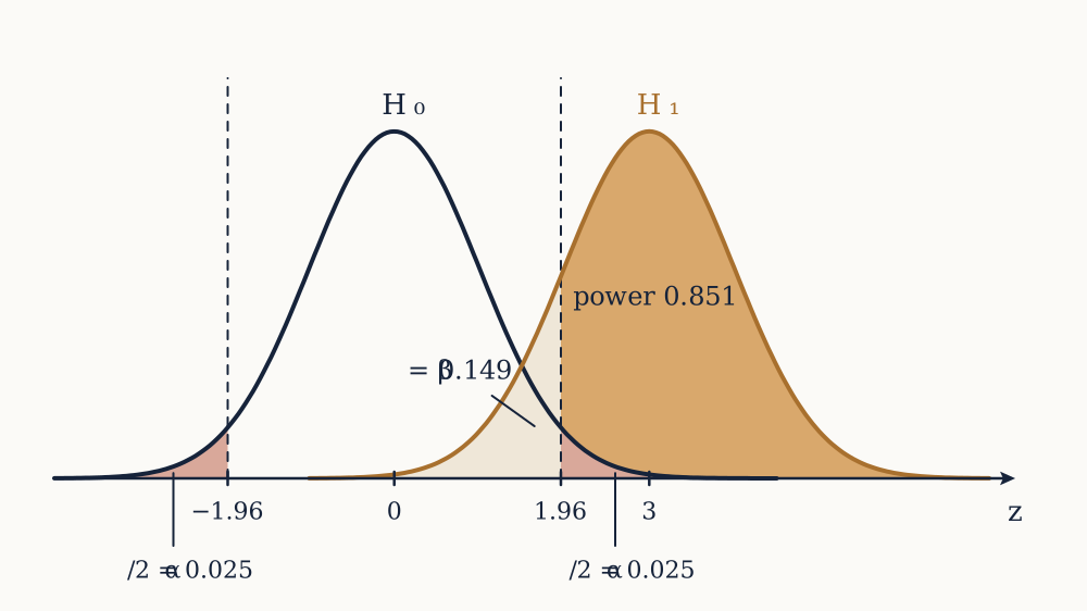
Example. A study of 100 observations tests a two-sided hypothesis at $α = 0.05$ , and the true standardised effect is $d = 0.3$ . What is the power?

$λ = 0.3 \sqrt{100} = 3$ , so the power is $Φ (3 - 1.96) = Φ (1.04) = 0.851$ . The study detects this effect about 85 times in 100, and misses it 15 times.

Now you. What is the power of the same study if the true effect is only $d = 0.2$ ?

Answer

$λ = 0.2 (10) = 2$ , so the power is $Φ (2 - 1.96) = Φ (0.04) = 0.516$ . A smaller effect halves the detection rate: this study is a coin toss against a $d = 0.2$ effect.

Sample size by inversion

Design usually runs the other way: fix the power you want and solve for $n$ . Dropping the negligible term, power $= 1 - β$ requires $λ - z_{1 - α / 2} = z_{1 - β}$ , so $λ = z_{1 - α / 2} + z_{1 - β}$ and

n = \frac{(z_{1 - α / 2} + z_{1 - β})^{2}}{d^{2}}

At the standard $α = 0.05$ and 80 per cent power, the multipliers are 1.960 and 0.8416, whose sum squared is 7.849, so $n = 7.849 / d^{2}$ . That gives 13 observations for $d = 0.8$ , 32 for $d = 0.5$ , 88 for $d = 0.3$ and 197 for $d = 0.2$ .

Two things follow immediately. The sample size scales as $1 / d^{2}$ , so halving the effect you want to detect quadruples the study, which is the $\sqrt{n}$ law once more. And 80 per cent power, the usual target, means accepting a one-in-five chance of missing a real effect of exactly the size you designed for, which is a much weaker standard than the 5 per cent on the other side and is rarely presented that way.

The honest version of this calculation requires committing in advance to the smallest effect worth detecting, which is a scientific or clinical judgement rather than a statistical one. Running it backwards, plugging in whatever $n$ is affordable and reporting the effect that would give 80 per cent power, is a common and useless ritual: it names an effect the study can detect, not one anybody had reason to expect.

Example. How many observations are needed for 80 per cent power against a standardised effect of $d = 0.5$ , two-sided at $α = 0.05$ ?

$n = 7.849 / 0.25 = 31.4$ , so 32 observations. This is the calculation behind the folklore that "about 30" is enough, and it is enough only for an effect of half a standard deviation, which is large.

Now you. How many are needed for the same power against $d = 0.2$ ?

Answer

$n = 7.849 / 0.04 = 196.2$ , so 197 observations. Two and a half times the effect size costs six times the sample.

The winner's curse

Here is the result that changes how published findings should be read. Suppose a real effect $δ$ exists and the study has low power. Most of the time it will fail to reach significance. On the occasions when it does reach significance, the estimate must have been unusually large, because that is the only way an underpowered study crosses the threshold. So the published estimates, which are the significant ones, are systematically too big.

The size of the exaggeration can be computed from a truncated normal. Let the estimate be normal around $δ$ , and condition on it exceeding $1.96$ standard errors. The ratio of the expected published estimate to the true effect, sometimes called the exaggeration ratio or type M error, works out to

Power	Exaggeration ratio
0.10	3.72
0.20	2.26
0.50	1.41
0.80	1.13

A study with 20 per cent power that reports a significant effect is reporting, on average, something 2.3 times the truth. At 10 per cent power it is nearly four times. This is not fraud or incompetence; it is what the threshold does to a noisy estimate, and it happens to a perfectly executed study.

That matters because low power is normal. Button and colleagues surveyed neuroscience in 2013 and estimated the median power of studies in that literature at about 21 per cent. A field working at 20 per cent power publishes findings that are real about as often as not and roughly twice as large as they should be, and then a better-powered replication finds a smaller effect and is read as a failure to replicate.

Example. A study has 20 per cent power against the true effect. It reports a significant result of $d = 0.60$ . What is a reasonable guess at the true effect?

Dividing by the exaggeration ratio of 2.26 gives about $d = 0.27$ . The published number is not wrong arithmetic; it is a biased sample of the estimates that study could have produced, and the bias is a property of the publication rule rather than of the analysis.

Now you. A well-powered study, 80 per cent, reports $d = 0.60$ . What correction applies?

Answer

Dividing by 1.13 gives about $d = 0.53$ , a correction of 12 per cent rather than a factor of two. High power is what makes a published estimate approximately trustworthy, which is a second and better reason to want it.

How often is a significant finding true

Combine power with the base rate, and the result is the calculation the probability course did for medical screening, applied to research itself. Suppose a fraction $π$ of the hypotheses a field investigates are true, and studies run at level $α$ with power $1 - β$ . Then among all findings that reach significance, the fraction that are true is

PPV = \frac{π (1 - β)}{π (1 - β) + (1 - π) α}

which is Bayes' theorem with "true hypothesis" in place of "has the disease".

Take a field where one hypothesis in ten is true, so $π = 0.1$ . With 80 per cent power, the PPV is $0.08 / (0.08 + 0.045) = 0.64$ : about a third of significant findings are false. With 20 per cent power it falls to $0.02 / (0.02 + 0.045) = 0.31$ , so most published significant findings in that field are wrong. This is the core of John Ioannidis's 2005 argument, and every input to it is a quantity the field controls: the ambition of the hypotheses, the power of the studies, and the threshold.

Notice which lever moves the answer most. Raising power from 0.2 to 0.8 quadruples the numerator; tightening $α$ from 0.05 to 0.005 divides the second denominator term by ten. Both help, and neither helps if the reported $p$ -values came from an analysis chosen after seeing the data, which is the subject of the final lesson.

What follows from all this

Three practical rules come out of this lesson, and they are the ones that survive contact with real work.

Decide the smallest effect worth detecting before the study, and compute the sample size from it. If the required $n$ is unaffordable, that is information: the study as conceived cannot answer the question, and running it anyway produces a result whose most likely outcomes are a null finding that means nothing and a significant one that is inflated.

Report the estimate and its interval rather than the verdict. A wide interval around a large point estimate is visibly uninformative, whereas " $p = 0.03$ " from the same data looks like a discovery.

Read a surprising result from a small study as an overestimate by default. The exaggeration ratios above give the size of the discount, and it depends only on the power, which can be reconstructed roughly from the reported interval.

All of this concerned one sample compared with a fixed value. Almost every real question compares two groups instead, which changes the arithmetic in ways worth doing carefully, and that is next.