Equilibrium, surplus and taxes

Demand says what buyers will take at each price and supply says what sellers will offer, and the market price is the one number at which those two answers agree.

Marshall's scissors metaphor is the right one: asking whether demand or supply determines the price is like asking which blade of a pair of scissors cuts the paper. This lesson finds the crossing point, defines what each side gains from trading there, establishes the sense in which that quantity is the best one, and then breaks it with a tax to see what breaking it costs.

Equilibrium and the adjustment story

Take demand $Q_{d} = 120 - 2 p$ and supply $Q_{s} = 3 p - 30$ , both in units per week with $p$ in pounds. Setting them equal, $120 - 2 p = 3 p - 30$ , so $5 p = 150$ and $p = £ 30$ , with $Q = 60$ units.

The claim that the market goes there needs an argument, and the standard one is about disequilibrium. At £40 supply is 90 and demand is 40, so 50 units go unsold, and sellers holding stock they cannot shift cut prices. At £20 demand is 80 and supply is 30, so buyers who cannot get the good bid the price up. Only at £30 does nobody have a reason to move. This is a story about incentives to change price rather than a theorem, and it can fail: markets with long production lags can oscillate around the equilibrium rather than converge to it, which is the cobweb model, and agricultural prices genuinely do this.

Comparative statics is the routine use of the model. A shift of one curve moves the equilibrium along the other, so the direction of the price and quantity changes identifies which curve moved. A bad harvest shifts supply left, raising price and cutting quantity. A fashion for a good shifts demand right, raising both. Price and quantity moving in opposite directions is the signature of a supply shift; in the same direction, a demand shift. That inference is the closest this apparatus gets to reading history off a price series, and it is also why the identification problem from the elasticity lesson is hard: without knowing which curve moved, the data say nothing about either.

Consumer and producer surplus

Trade makes both sides better off, and the areas on the diagram measure by how much. Jules Dupuit constructed the first such measure in 1844, while working out whether a bridge was worth building, and Marshall named it in 1890.

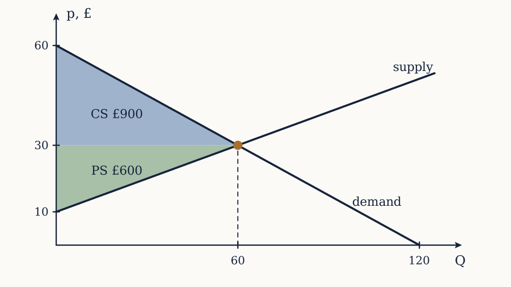
Read the demand curve as a marginal willingness to pay: the height at quantity $q$ is what the buyer of the $q$ th unit would have paid at most. Everyone pays the market price, so each buyer's gain is the gap between their valuation and the price, and consumer surplus is the integral of that gap:

CS = \int_{0}^{Q} (p_{d} (q) - p^{*}) d q

Geometrically it is the area below the demand curve and above the price. Similarly, the height of the supply curve at $q$ is the marginal cost of the $q$ th unit, so producer surplus is the area above the supply curve and below the price, which equals revenue minus variable cost. Note that producer surplus is not profit: it exceeds profit by the fixed cost, since fixed costs never appear in a supply curve.

Example. For the market above, compute consumer and producer surplus at the equilibrium.

Inverting demand, $p = 60 - Q / 2$ , so the choke price is £60 and the demand curve meets the axis there. Consumer surplus is the triangle of height $60 - 30 = £ 30$ and base 60 units, giving $\frac{12}{\times} 60 \times 30 = £ 900$ a week. Inverting supply, $p = 10 + Q / 3$ , so the lowest price at which anything is supplied is £10, and producer surplus is $\frac{12}{\times} 60 \times 20 = £ 600$ . Total surplus is £1500.

Now you. A market has $Q_{d} = 200 - 4 p$ and $Q_{s} = 4 p - 40$ . Find the equilibrium and both surpluses.

Answer

$200 - 4 p = 4 p - 40$ gives $p = £ 30$ and $Q = 80$ . Inverse demand is $p = 50 - Q / 4$ with a choke price of £50, so consumer surplus is $\frac{12}{\times} 80 \times 20 = £ 800$ . Inverse supply is $p = 10 + Q / 4$ , so producer surplus is also $\frac{12}{\times} 80 \times 20 = £ 800$ . Total surplus is £1600, split evenly because the two curves have the same slope.

Why the competitive quantity is the right one

Now the result that the rest of the course is measured against. Consider any quantity $q$ and ask whether producing one more unit raises total surplus. The buyer values it at $p_{d} (q)$ , the demand curve height. It costs $p_{s} (q)$ to make, the supply curve height. The unit is worth making exactly when $p_{d} (q) > p_{s} (q)$ , so surplus rises with output while demand lies above supply and falls once supply lies above demand. Total surplus is therefore maximised where the two curves cross, which is the competitive equilibrium.

Said in terms of the firm's condition, the competitive outcome has $p = MC$ , and price is marginal value while marginal cost is marginal cost, so the last unit produced is worth exactly what it costs. That is the whole content of the efficiency claim. Every unit whose value exceeds its cost gets made, and no unit whose cost exceeds its value does.

Three qualifications keep this from meaning more than it does, and all three become lessons later.

Total surplus counts a pound the same whoever receives it. A change that takes £100 from a poor buyer and gives £120 to a rich seller raises total surplus, and calling that an improvement is a normative judgement the model does not make and cannot support. Efficiency is a statement about the size of the pie only.

The demand curve measures willingness to pay, which is bounded by ability to pay. Somebody with no money has no willingness to pay for anything, and their needs do not appear on the diagram at all.

And the result assumes every cost and benefit falls on the two parties trading. When it does not, the supply curve is not marginal social cost and the whole argument fails, which is what the externalities lesson is about.

A tax drives a wedge

Put a tax of $t$ per unit on sellers. They now need $t$ more than before to supply any given quantity, so the price buyers pay and the price sellers receive differ by exactly $t$ : $p_{b} - p_{s} = t$ . Which side the tax is legally levied on makes no difference at all to the outcome, since the equations only contain the wedge. This is the irrelevance of statutory incidence, and it is one of the most robust and least believed results in the subject. Jonathan Gruber's study of the large payroll tax cuts in Chile between 1981 and 1986 found essentially full shifting into wages, exactly as the model says: who writes the cheque does not decide who bears the burden.

Example. The market $Q_{d} = 120 - 2 p$ , $Q_{s} = 3 p - 30$ faces a tax of £10 per unit. Find the two prices, the quantity, the revenue, and how the burden splits.

With $p_{s} = p_{b} - 10$ , supply becomes $Q_{s} = 3 (p_{b} - 10) - 30 = 3 p_{b} - 60$ . Setting that equal to demand, $120 - 2 p_{b} = 3 p_{b} - 60$ , so $5 p_{b} = 180$ and $p_{b} = £ 36$ , $p_{s} = £ 26$ , and $Q = 48$ . Buyers pay £6 more than before, sellers receive £4 less, so buyers bear 60 per cent of the tax. Revenue is $10 \times 48 = £ 480$ a week.

The 60 per cent is predictable from elasticities. At the original equilibrium, $ε_{d} = - 2 \times 30 / 60 = - 1$ and $ε_{s} = 3 \times 30 / 60 = 1.5$ . The buyers' share is $ε_{s} / (ε_{s} + | ε_{d} |) = 1.5 / 2.5 = 0.6$ . The rule behind it is simple: the more inelastic side bears more of the tax, because being inelastic means having fewer alternatives to escape into.

Now you. The market $Q_{d} = 200 - 4 p$ , $Q_{s} = 4 p - 40$ faces a tax of £8 per unit. Find the two prices, the quantity, and the split.

Answer

Supply becomes $4 (p_{b} - 8) - 40 = 4 p_{b} - 72$ , and $200 - 4 p_{b} = 4 p_{b} - 72$ gives $p_{b} = £ 34$ , $p_{s} = £ 26$ and $Q = 64$ . The burden splits exactly evenly, £4 each way, because the elasticities are equal in magnitude at the original equilibrium: both are 1.5. Revenue is $8 \times 64 = £ 512$ .

Deadweight loss grows with the square of the tax

The tax cut output from 60 to 48. Those twelve units were worth more to buyers than they cost to make, and now they are not produced. Their lost surplus is the triangle between the two curves over the missing range, with height $t$ and base $Δ Q$ :

DWL = \frac{12}{} t Δ Q

Here that is $\frac{12}{\times} 10 \times 12 = £ 60$ a week. Check the accounting: consumer surplus falls from £900 to $\frac{12}{\times} 48 \times 24 = £ 576$ , and producer surplus from £600 to $\frac{12}{\times} 48 \times 16 = £ 384$ . The two losses sum to $324 + 216 = £ 540$ , of which £480 arrives as government revenue and £60 goes nowhere. That £60 is the deadweight loss, or Harberger triangle after Arnold Harberger's 1954 use of it.

The important structural fact is that $Δ Q$ is itself proportional to $t$ , so deadweight loss is proportional to $t^{2}$ . Doubling a tax quadruples its excess burden. On this market $Δ Q = 1.2 t$ , so $DWL = 0.6 t^{2}$ .

Example. Confirm the square rule by computing the deadweight loss of a £20 tax on the same market.

Supply becomes $3 p_{b} - 90$ , and $120 - 2 p_{b} = 3 p_{b} - 90$ gives $p_{b} = £ 42$ , $p_{s} = £ 22$ and $Q = 36$ . Deadweight loss is $\frac{12}{\times} 20 \times 24 = £ 240$ , which is four times the £60 from the £10 tax, as $0.6 \times 400$ requires. Revenue is $20 \times 36 = £ 720$ .

Now you. Find the price, quantity, revenue and deadweight loss for a £30 tax on the same market, and compare the revenue with that of the £20 tax.

Answer

Supply becomes $3 p_{b} - 120$ , giving $p_{b} = £ 48$ , $p_{s} = £ 18$ and $Q = 24$ . Deadweight loss is $\frac{12}{\times} 30 \times 36 = £ 540$ , which is nine times the £10 figure. Revenue is $30 \times 24 = £ 720$ , exactly the same as the £20 tax raised, while the deadweight loss has more than doubled. Revenue as a function of the tax rate is $t (60 - 1.2 t)$ , which peaks at $t = £ 25$ with £750, so a £30 tax is on the wrong side of the peak.

Two policy conclusions come straight out of the algebra. Since excess burden grows with the square of the rate, several small taxes on different goods cost less in total than one large tax raising the same money, which is the case for a broad base and low rates. And since deadweight loss depends on how much the quantity moves, taxing inelastic things is cheaper in efficiency terms, which is the Ramsey rule of 1927 and also, uncomfortably, an argument for taxing necessities.

Floors and ceilings

A price ceiling below equilibrium creates excess demand, and a price floor above it creates excess supply. The surplus arithmetic is the same as for a tax except that no revenue is raised, so the whole reduction in trade is lost, and it is worse still if the units that do get traded are not the ones with the highest value or the lowest cost.

Rent control is the standard case and the evidence is more interesting than either side usually admits. Rebecca Diamond, Tim McQuade and Franklin Qian studied San Francisco's 1994 extension of rent control to small multi-family buildings and found that it delivered substantial benefits to the tenants covered, who were significantly more likely to stay in the city, while landlords responded by converting and redeveloping properties enough to cut the rental housing supply of affected buildings by about 15 per cent, raising rents city-wide. Both effects are real, they fall on different people, and the surplus arithmetic on its own cannot say which matters more. That is exactly the limit of this apparatus.

The efficiency benchmark is now established and one way of breaking it, taxation, has been measured. The next three lessons break it in a more fundamental way, by dropping the assumption that firms take the price as given.