Monopoly

Every result in the previous lesson rested on firms taking the price as given, and this lesson drops that single assumption and keeps everything else.

A monopoly is a market with one seller and no close substitute. What makes it a different problem is not size or wickedness but the shape of the demand curve the firm faces: it is the market demand curve, sloping downwards, so selling more requires charging less. That one change propagates through the whole analysis and produces a quantity below the efficient one, which is the first genuine failure of the competitive benchmark.

Where a monopoly comes from

Monopoly needs a barrier to entry, otherwise the profits attract competitors and the situation ends. Four kinds are worth distinguishing.

Legal barriers are the commonest and the most deliberate. A patent grants exclusive rights for twenty years from filing under the international agreement of 1994, on the explicit argument that temporary monopoly is the price of getting the invention at all. Copyrights, broadcast licences and taxi medallions do the same thing with less justification.

Control of a scarce input is the classic private route. De Beers held roughly 80 per cent of world rough diamond supply for much of the twentieth century by buying up production and stockpiling it, and its share fell below half in the 2000s once Russian, Australian and Canadian output found other channels. That trajectory is the normal one: input monopolies are eroded by discovery.

Natural monopoly arises when one firm can supply the whole market more cheaply than two can, which happens whenever average cost is still falling at the scale of total demand. Water distribution, electricity transmission and rail track are the standard examples, and this case gets a section of its own below because it cannot be fixed by encouraging entry.

Network effects make a product more valuable the more people use it, so an early lead compounds. This is the modern case and it is genuinely different from the others, since the barrier is created by the customers rather than by the firm.

Marginal revenue lies below price

Here is the whole of monopoly in one derivation. Revenue is $R = p (q) q$ , where $p (q)$ is inverse demand. Differentiate with the product rule:

MR = \frac{d R}{d q} = p (q) + q \frac{d p}{d q}

The first term is the money from the extra unit. The second is negative, because selling the extra unit requires cutting the price on every unit already being sold. A price taker has $d p / d q = 0$ and the second term vanishes, which is why $MR = p$ there. For anyone else marginal revenue is strictly below price.

Factor out $p$ and the elasticity appears:

MR = p (1 + \frac{1}{ε})

This is worth reading carefully. If demand is inelastic, $| ε | < 1$ , then $1 + 1 / ε$ is negative and marginal revenue is negative: selling more actually reduces revenue. Since costs are positive, a monopolist never operates on the inelastic part of its demand curve. It would raise price, sell less, earn more and spend less. Any firm found pricing where demand is inelastic is either not a monopolist or not maximising.

For linear inverse demand $p = a - b q$ , revenue is $a q - b q^{2}$ and marginal revenue is $a - 2 b q$ : the same intercept and twice the slope. That doubling is worth memorising, since it makes every linear monopoly problem a two-line calculation.

The monopoly output

Profit maximisation is $MR = MC$ , exactly as for any firm. What differs is that marginal revenue is not the price, so the price ends up above marginal cost.

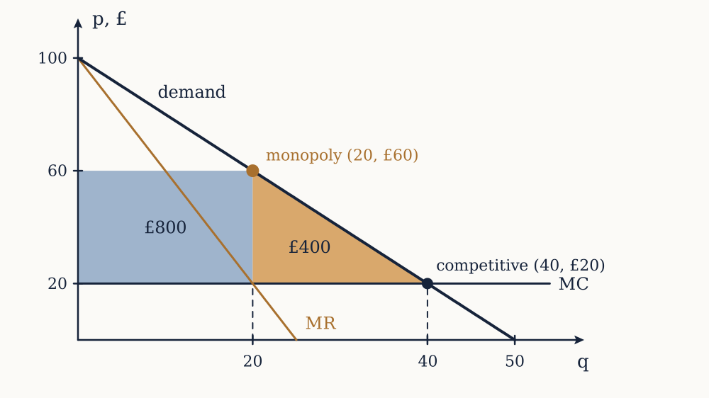
Example. A monopolist faces $p = 100 - 2 q$ and has $C (q) = 100 + 20 q$ . Find its output, price and profit, compare with the competitive outcome, and compute the deadweight loss.

Marginal revenue is $100 - 4 q$ and marginal cost is £20. Setting them equal, $100 - 4 q = 20$ , so $q = 20$ and $p = 100 - 40 = £ 60$ . Profit is $60 \times 20 - (100 + 400) = £ 700$ .

A competitive industry with the same costs would produce where $p = MC$ : $100 - 2 q = 20$ gives $q = 40$ at a price of £20. So the monopolist sells half as much at three times the price. The deadweight loss is the triangle between demand and marginal cost over the missing 20 units, $\frac{12}{\times} (60 - 20) \times (40 - 20) = £ 400$ a week. Consumer surplus falls from $\frac{12}{\times} 40 \times 80 = £ 1600$ to $\frac{12}{\times} 20 \times 40 = £ 400$ , so consumers lose £1200, of which £800 is transferred to the firm as profit and £400 is destroyed.

Now you. A monopolist faces $p = 120 - 3 q$ with $C (q) = 200 + 30 q$ . Find output, price, profit and deadweight loss.

Answer

Marginal revenue is $120 - 6 q$ , so $120 - 6 q = 30$ gives $q = 15$ and $p = £ 75$ . Profit is $75 \times 15 - (200 + 450) = £ 475$ . The competitive quantity solves $120 - 3 q = 30$ , giving $q = 30$ , so the deadweight loss is $\frac{12}{\times} (75 - 30) \times (30 - 15) = £ 337.50$ .

The markup rule

Substituting $MR = p (1 + 1 / ε)$ into $MR = MC$ and rearranging gives the result in its most useful form:

\frac{p - MC}{p} = - \frac{1}{ε}

The left side is the Lerner index, defined by Abba Lerner in 1934 as the fraction of price that is markup over marginal cost. It is the standard measure of market power, running from 0 for a price taker to 1 as elasticity approaches zero. The result says the markup is determined entirely by the elasticity of demand at the chosen point, and by nothing else: not by cost, not by firm size, not by how many competitors are visible.

In the worked example, price is £60 and marginal cost £20, so the Lerner index is $40 / 60 = 0.667$ . The elasticity at that point is $(- 1 / 2) (60 / 20) = - 1.5$ , and $- 1 / (- 1.5) = 0.667$ . The two agree, as they must.

The rule also explains why monopolists do not charge "as much as possible". There is no such quantity. The firm charges the amount that makes the elasticity consistent with its costs, which for a low-cost firm facing elastic demand can be a very modest markup.

A monopolist has no supply curve

This sounds like a technicality and is not. A supply curve answers "how much would you produce at price $p$ ", and that question is meaningless for a monopolist, because it chooses the price rather than reading it off the market. Its output depends on the whole shape of demand, not on one point of it, and two different demand curves passing through the same price and quantity can produce different monopoly outputs. The supply curve is an artefact of price taking, and dropping price taking dissolves it.

Natural monopoly, and the trouble with regulating it

When average cost falls over the whole range of demand, the efficient number of firms is one, and the competitive prescription $p = MC$ becomes a trap. With falling average cost, marginal cost lies below average cost everywhere, so a firm charging marginal cost loses money on every unit and cannot survive without a subsidy.

Example. A water utility faces $p = 70 - 0.5 q$ and has $C (q) = 1600 + 10 q$ . Find the unregulated monopoly outcome, what happens under marginal cost pricing, and what price covers costs exactly.

Unregulated: $MR = 70 - q = 10$ , so $q = 60$ and $p = £ 40$ , with profit $2400 - 2200 = £ 200$ .

Marginal cost pricing: $p = £ 10$ gives $q = 120$ , revenue £1200 against costs of $1600 + 1200 = £ 2800$ , a loss of £1600. That loss is exactly the fixed cost, which is what constant marginal cost guarantees. The efficient quantity is unfinanceable at the efficient price.

Average cost pricing: set $70 - 0.5 q = 1600 / q + 10$ , which rearranges to $q^{2} - 120 q + 3200 = 0$ with roots 40 and 80. The regulator wants the larger one, so $q = 80$ at $p = £ 30$ , where average cost is $1600 / 80 + 10 = £ 30$ exactly. The firm breaks even and output is two thirds of the efficient level.

Now you. For that utility, compute the deadweight loss under average cost pricing and under unregulated monopoly.

Answer

The efficient quantity is 120. Under average cost pricing, $q = 80$ and $p = £ 30$ , so the loss is $\frac{12}{\times} (30 - 10) \times (120 - 80) = £ 400$ . Unregulated, $q = 60$ and $p = £ 40$ , so the loss is $\frac{12}{\times} (40 - 10) \times (120 - 60) = £ 900$ . Regulation more than halves the loss without eliminating it, which is the honest description of what utility regulation achieves.

Average cost pricing, or rate-of-return regulation, is what most utility regulators actually do, and it has a well documented side effect. Harvey Averch and Leland Johnson showed in 1962 that a firm allowed a fixed return on its capital base has an incentive to enlarge that base, choosing a more capital-intensive method than cost minimisation would pick. Frank Ramsey's 1927 alternative, spreading the fixed cost across products in inverse proportion to their elasticities, minimises the deadweight loss subject to breaking even, and is used in rail and postal pricing.

Price discrimination

A single price leaves money on the table: buyers who would have paid more get a surplus, and buyers who would have paid a little above marginal cost are not served at all. Price discrimination is charging different prices to different buyers for reasons unrelated to cost. It requires market power, some way of telling buyers apart, and a way to prevent resale.

First degree, or perfect, discrimination charges each buyer their full willingness to pay. Output rises to the efficient level, because every unit worth more than marginal cost now gets sold, and the deadweight loss vanishes entirely. All of the surplus goes to the seller. This is the sharpest illustration in the subject that efficiency and fairness are separate axes.

Second degree offers a menu and lets buyers sort themselves: bulk discounts, first and standard class, advance purchase fares. The seller does not know who is who, so the menu has to be designed so that each type prefers the option intended for it.

Third degree charges different prices to identifiable groups: student tickets, senior discounts, regional pricing. Here the arithmetic is clean, because the firm simply runs a separate monopoly problem in each market with the same marginal cost.

Example. A firm with constant marginal cost £20 sells in two separated markets, $p_{1} = 100 - 2 q_{1}$ and $p_{2} = 80 - q_{2}$ . Find its prices, and check them against the elasticities.

In market 1, $100 - 4 q_{1} = 20$ gives $q_{1} = 20$ and $p_{1} = £ 60$ . In market 2, $80 - 2 q_{2} = 20$ gives $q_{2} = 30$ and $p_{2} = £ 50$ . Total profit is $1200 + 1500 - 1000 = £ 1700$ . The elasticities are $- 1.5$ in market 1 and $- 1.67$ in market 2, so the lower price goes to the more elastic market, exactly as the markup rule requires. Forced to charge one price, the firm would set £53.33 and earn £1666.67, so discrimination is worth £33.33 a week to it.

Now you. The same two markets, but marginal cost rises to £30. Find the two prices and the total profit.

Answer

Market 1: $100 - 4 q_{1} = 30$ gives $q_{1} = 17.5$ and $p_{1} = £ 65$ . Market 2: $80 - 2 q_{2} = 30$ gives $q_{2} = 25$ and $p_{2} = £ 55$ . Profit is $1137.50 + 1375 - 1275 = £ 1237.50$ . Both prices rose by less than the £10 cost increase, which is the general pattern for linear demand: a monopolist passes through only half of a constant marginal cost rise.

Whether third-degree discrimination helps or hurts overall is genuinely ambiguous. It raises output in the market that would otherwise be priced out and cuts it in the other, so the sign of the welfare change depends on the curvature of the two demands. Regional pricing of medicines is the case where it matters most: uniform world pricing would be simpler and would leave poorer countries unserved.

How much does monopoly actually cost?

The triangle is easy to draw and hard to measure. Arnold Harberger tried it for United States manufacturing in 1954 and found a deadweight loss of about 0.1 per cent of national income, an answer so small it embarrassed the profession and set off a literature. Later work using different methods, notably Keith Cowling and Dennis Mueller in 1978, put the figure at several per cent by counting advertising and lobbying as part of the cost and by measuring markups firm by firm rather than industry by industry.

Both approaches miss things that are probably larger than the triangle. Resources spent obtaining and defending a monopoly, from lobbying to patent litigation, are a real cost that no triangle captures. So is the tendency of a firm without competitive pressure to run at higher cost than necessary, which raises the marginal cost curve rather than moving along it. And in the other direction, Joseph Schumpeter argued in 1942 that the prospect of monopoly profit is precisely what pays for innovation, so a snapshot comparison against a competitive counterfactual measures the wrong thing entirely.

Monopoly and perfect competition are the two endpoints, and almost every real market is between them. The next lesson works out what happens with a handful of firms, where each one's best move depends on what the others do.