Systems and the phase plane

Two tanks feeding each other, two masses on a shared spring, and a predator with its prey all have something the equations so far cannot express: more than one unknown function, each depending on the others.

Such a model is a system of differential equations, and the useful discovery is that systems are not a complication added to the subject but the natural home of it. Writing a second order equation as a pair of first order ones costs nothing, gains a picture, and is what every numerical solver does internally.

Everything is a first order system

Take any equation of order $n$ , solved for the highest derivative. Name the unknown and its derivatives as separate variables: for $y'' + 3 y' + 2 y = \cos t$ , put $x_{1} = y$ and $x_{2} = y'$ . Then

x_{1}' = x_{2}, x_{2}' = - 3 x_{2} - 2 x_{1} + \cos t

a pair of first order equations. The first is a definition and the second is the original equation rewritten. Nothing is lost, and the initial conditions $y (0)$ , $y' (0)$ become the two starting values $x_{1} (0)$ , $x_{2} (0)$ , which is why they were needed.

The pair $(x_{1}, x_{2})$ is the state: the smallest collection of numbers that determines the future. For a mechanical system it is position and velocity, for a circuit it is capacitor voltage and inductor current. Once the state is identified, the equation says how it changes, and that is all a differential equation ever says.

Example. Write $y''' - 2 y'' + y' - 5 y = e^{t}$ as a first order system.

Put $x_{1} = y$ , $x_{2} = y'$ , $x_{3} = y''$ . Then $x_{1}' = x_{2}$ , $x_{2}' = x_{3}$ , and solving the original for $y'''$ gives $x_{3}' = 2 x_{3} - x_{2} + 5 x_{1} + e^{t}$ . Three first order equations, three initial values.

Now you. Write the driven oscillator $2 y'' + 6 y' + 8 y = 3 \sin t$ as a first order system.

Answer

Divide by $2$ first: $y'' + 3 y' + 4 y = 1.5 \sin t$ . With $x_{1} = y$ and $x_{2} = y'$ , the system is $x_{1}' = x_{2}$ and $x_{2}' = - 3 x_{2} - 4 x_{1} + 1.5 \sin t$ .

The phase plane

For a system of two equations that do not mention $t$ explicitly,

x' = f (x, y), y' = g (x, y)

the state is a point in the plane and the equations give its velocity vector at every point. A solution traces a curve, its trajectory or orbit, and the plane filled with trajectories is the phase portrait. This is the two dimensional relative of the phase line, and it inherits its main property: trajectories cannot cross, since a crossing point would have two different futures, which uniqueness forbids.

What is gained by discarding $t$ is that a whole family of behaviours becomes one picture. What is lost is the timing: a portrait shows a closed loop without saying whether the circuit takes a second or a year.

The oscillator of the last three lessons is the first example. With $x$ the displacement and $v$ the velocity,

x' = v, v' = - ω_{0}^{2} x - 2 ζ ω_{0} v

An undamped oscillator conserves energy, ${\frac{12}{v}}^{2} + {\frac{12}{ω}}_{0}^{2} x^{2}$ , so its trajectories are the level curves of that quantity: ellipses around the origin, traversed clockwise, closed because the motion repeats. Add light damping and each loop falls slightly inside the previous one, making an inward spiral. Increase the damping past critical and the spiral straightens into a direct approach along a preferred direction. The three regimes of the eighth lesson are three shapes in one plane.

Linear systems, solved by the same guess

Take the constant coefficient linear case, which will turn out to describe every equilibrium's neighbourhood:

x' = a x + b y, y' = c x + d y

Try the same thing that worked before, a solution where both variables share one exponential: $x = p e^{λ t}$ and $y = q e^{λ t}$ , with the constants $p$ and $q$ giving the direction. Substituting and cancelling the exponential,

λ p = a p + b q, λ q = c p + d q

which in the language of the linear algebra course says that $λ$ is an eigenvalue and the direction $(p, q)$ its eigenvector. Rearranged, $(a - λ) p + b q = 0$ and $c p + (d - λ) q = 0$ . These have a solution other than $p = q = 0$ only when the two lines coincide, that is when $(a - λ) (d - λ) - b c = 0$ . Expanding,

λ^{2} - τ λ + Δ = 0, τ = a + d, Δ = a d - b c

with $τ$ the trace and $Δ$ the determinant. So a two variable linear system is again governed by a quadratic, whose two roots give two exponential solutions, and the general solution is their combination with two arbitrary constants, matching the two initial values.

The direction that goes with a root follows from either equation: $q / p = (λ - a) / b$ when $b \neq 0$ . Along that direction the system moves purely outwards or inwards, with no turning, which makes eigenvector directions the skeleton of the portrait.

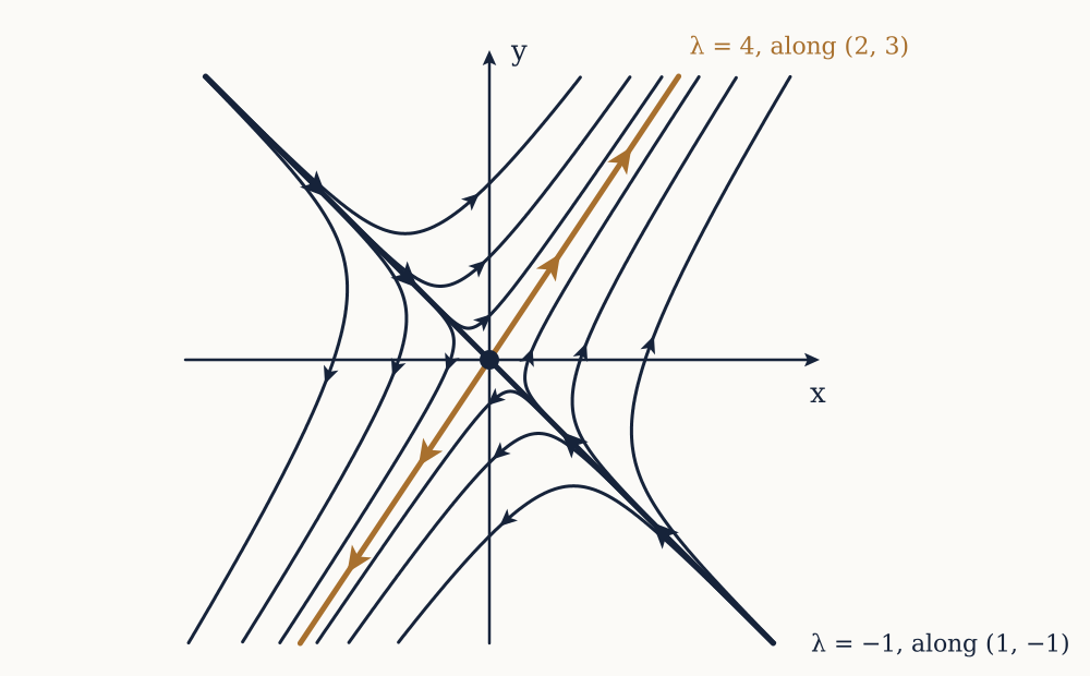
Example. Classify and solve $x' = x + 2 y$ , $y' = 3 x + 2 y$ .

Here $τ = 3$ and $Δ = 2 - 6 = - 4$ , so $λ^{2} - 3 λ - 4 = 0$ and $λ = 4$ or $λ = - 1$ . Real roots of opposite sign. For $λ = 4$ , $q / p = (4 - 1) / 2 = 1.5$ , so the direction is along $(2, 3)$ ; for $λ = - 1$ , $q / p = (- 1 - 1) / 2 = - 1$ , direction $(1, - 1)$ . The general solution is

x = 2 c_{1} e^{4 t} + c_{2} e^{- t}, y = 3 c_{1} e^{4 t} - c_{2} e^{- t}

Every trajectory not exactly on the line $y = - x$ eventually runs off along $(2, 3)$ . The origin is a saddle: attracting along one direction, repelling along another, and unstable overall.

Now you. Classify and find the eigenvalues of $x' = - 3 x + y$ , $y' = x - 3 y$ .

Answer

$τ = - 6$ and $Δ = 9 - 1 = 8$ , so $λ^{2} + 6 λ + 8 = 0$ and $λ = - 2$ or $λ = - 4$ . Both real and negative, so the origin is a stable node and every trajectory approaches it, eventually along the direction belonging to $λ = - 2$ , the slower root.

The four portraits

The discriminant $τ^{2} - 4 Δ$ and the signs of $τ$ and $Δ$ classify every linear system in the plane, and there are only four generic pictures.

If $Δ < 0$ the roots are real with opposite signs, and the origin is a saddle, always unstable. If $Δ > 0$ and $τ^{2} > 4 Δ$ the roots are real with the same sign, and the origin is a node, stable when $τ < 0$ and unstable when $τ > 0$ . If $τ^{2} < 4 Δ$ the roots are complex, and the origin is a spiral, stable when $τ < 0$ and unstable when $τ > 0$ . If $τ = 0$ with $Δ > 0$ the roots are purely imaginary and the origin is a centre, surrounded by closed loops, neither attracting nor repelling.

Two conclusions are worth stating plainly. Stability requires $τ < 0$ and $Δ > 0$ , a two line test that needs no root finding at all. And the centre is the delicate case, because it needs $τ$ to be exactly zero; any perturbation of the coefficients turns it into a spiral one way or the other. That fragility matters in the next lesson.

Two tanks

Systems arise most naturally when several reservoirs exchange contents. Take two tanks of $100$ litres each. Fresh water enters tank A at $5$ litres per minute, brine flows from A to B at $10$ litres per minute, from B back to A at $5$ litres per minute, and leaves B at $10$ litres per minute. Every volume stays constant. With $x$ and $y$ the salt masses in kilograms,

x' = - \frac{10}{100} x + \frac{5}{100} y = - 0.1 x + 0.05 y

y' = \frac{10}{100} x - \frac{10}{100} y = 0.1 x - 0.1 y

Example. Find the eigenvalues of that system and say what the tanks do.

$τ = - 0.2$ and $Δ = 0.01 - 0.005 = 0.005$ , so $λ^{2} + 0.2 λ + 0.005 = 0$ and $λ = (- 0.2 \pm \sqrt{0.04 - 0.02}) / 2 = - 0.029$ or $- 0.171$ per minute. Both real and negative, so the origin is a stable node: all the salt eventually washes out, whatever the starting amounts. The slow mode has time constant $1 / 0.029 = 34$ minutes and the fast one $1 / 0.171 = 5.9$ minutes, so after about twenty minutes only the slow mode is left and the two tanks empty together in fixed proportion, along that mode's direction. That is a general feature of coupled linear systems: they forget everything except their slowest mode.

Now you. The same tanks are run at double all the flow rates. Find the new eigenvalues.

Answer

Every coefficient doubles: $x' = - 0.2 x + 0.1 y$ and $y' = 0.2 x - 0.2 y$ . Then $τ = - 0.4$ and $Δ = 0.04 - 0.02 = 0.02$ , giving $λ = - 0.059$ and $- 0.341$ per minute, exactly twice the previous values. Doubling every flow halves every timescale and leaves the shape of the portrait unchanged.

Repeated roots and other degenerate cases

If $τ^{2} = 4 Δ$ the root is repeated. Sometimes the system still has two independent directions, in which case every direction is an eigenvector and the trajectories are straight lines through the origin, a star node, which happens only when $b = c = 0$ and $a = d$ . Otherwise there is one direction only, and the second solution acquires a factor of $t$ exactly as it did for a repeated characteristic root, producing a degenerate node whose trajectories all come in tangent to the single eigenvector direction.

If $Δ = 0$ one root is zero, and there is a whole line of equilibria rather than an isolated one. The system slides onto that line and stops somewhere along it, with the stopping point depending on the initial condition. This is what a system with no restoring force in one direction does, and it is the linear picture of a conserved quantity.

What this buys, and what it does not

Any system of two linear equations with constant coefficients is now completely solved and classified by two numbers. Since a second order equation is such a system, this includes everything in the last four lessons: the mass on a spring is a spiral when underdamped, a node when overdamped, and a centre when undamped, and the trace being $- 2 ζ ω_{0}$ says immediately that stability is exactly the condition $ζ > 0$ .

The method extends to $n$ variables, where the characteristic equation has degree $n$ and stability requires every root to have negative real part. The classification of portraits does not extend so simply, since three dimensions permit behaviour, including chaos, that a plane cannot contain.

What is missing is the nonlinear case, and it is most of nature. Predator and prey do not interact linearly, since the rate of predation depends on the product of the two populations. A pendulum's restoring force is $\sin θ$ rather than $θ$ . For those there are no eigenvalues and no general solution, but there is something almost as good: near any equilibrium the system looks linear, and the trace and determinant of that local approximation say what the portrait looks like there. The final lesson does that, and then asks what happens between the equilibria, where linearisation says nothing at all.