Nonlinear systems and what solutions say

Almost every equation worth writing down is nonlinear, and none of the machinery of the last six lessons applies to any of them.

Superposition is gone, so solutions cannot be added. The characteristic equation is gone, so there is no general solution to fit initial conditions to. What remains is the phase plane, and it turns out to be enough for a great deal: equilibria can be found and classified, conserved quantities constrain whole trajectories, and the questions worth asking about a physical system are usually answered without a formula at all. This lesson does that for three systems and then says where the programme ends.

Linearising at an equilibrium

For $x' = f (x, y)$ and $y' = g (x, y)$ , an equilibrium is a point where both $f$ and $g$ vanish, so the state does not move. Near it, expand both functions in a Taylor series and keep the linear terms. With $u$ and $v$ the displacements from the equilibrium $(x^{*}, y^{*})$ ,

u' \approx f_{x} u + f_{y} v, v' \approx g_{x} u + g_{y} v

where the four partial derivatives are evaluated at the equilibrium. That is a linear system of the kind fully classified in the previous lesson, with

τ = f_{x} + g_{y}, Δ = f_{x} g_{y} - f_{y} g_{x}

so the local portrait is a node, saddle, spiral or centre according to the same two numbers. The array of partial derivatives is the Jacobian, and the whole of local stability theory is contained in it.

The result is trustworthy with one important exception. Hartman and Grobman proved that whenever every eigenvalue has a nonzero real part, the nonlinear portrait near the equilibrium is a smooth distortion of the linear one, so saddles stay saddles and stable spirals stay stable spirals. When the linearisation gives a centre, with $τ = 0$ , the neglected quadratic terms decide, and they can make it a slow spiral either way. A centre in a linearisation is a question, not an answer.

Example. Two competing species obey $x' = x (3 - x - 2 y)$ and $y' = y (2 - x - y)$ . Classify the equilibrium at $(1, 1)$ .

First check it is one: $3 - 1 - 2 = 0$ and $2 - 1 - 1 = 0$ , so both rates vanish. Expanding, $f = 3 x - x^{2} - 2 x y$ and $g = 2 y - x y - y^{2}$ , so $f_{x} = 3 - 2 x - 2 y$ , $f_{y} = - 2 x$ , $g_{x} = - y$ and $g_{y} = 2 - x - 2 y$ . At $(1, 1)$ these are $- 1$ , $- 2$ , $- 1$ and $- 1$ . So $τ = - 2$ and $Δ = 1 - 2 = - 1$ . Since $Δ < 0$ the equilibrium is a saddle, hence unstable: coexistence at these numbers is possible in principle and destroyed by any disturbance, so one species or the other wins depending on the starting point.

Now you. Classify the equilibrium of the same system at $(3, 0)$ .

Answer

There $f_{x} = 3 - 6 - 0 = - 3$ , $f_{y} = - 6$ , $g_{x} = 0$ and $g_{y} = 2 - 3 - 0 = - 1$ . So $τ = - 4$ and $Δ = 3$ , with $τ^{2} - 4 Δ = 4 > 0$ : a stable node. The state where the first species holds the ground alone is stable against a small invasion by the second.

The pendulum, exactly

A rigid pendulum of length $L$ obeys $θ'' = - (g / L) \sin θ$ , which the eighth lesson linearised to $θ'' = - (g / L) θ$ and never revisited. Written as a system with $ω = θ'$ ,

θ' = ω, ω' = - \frac{g}{L} \sin θ

Equilibria occur where $ω = 0$ and $\sin θ = 0$ , so at $θ = 0$ , hanging down, and at $θ = π$ , balanced upright, repeating every $2 π$ . Linearising at the bottom gives $τ = 0$ and $Δ = g / L > 0$ , a centre, with the small oscillation frequency $ω_{0} = \sqrt{g / L}$ recovered. Linearising at the top gives $Δ = - g / L < 0$ , a saddle, which is the mathematical statement that an inverted pendulum falls.

The centre is exactly the case linearisation cannot settle, so use energy instead. Multiplying the equation by $θ'$ and integrating gives the conserved quantity

E = {\frac{12}{ω}}^{2} - \frac{g}{L} \cos θ

which is the energy per unit moment of inertia. Every trajectory lies on a level curve of $E$ , and that settles the global picture without any solving. Low energy gives closed loops around the bottom: genuine oscillation, so the centre is a true centre here, protected by the conservation law rather than by the linearisation. High energy gives curves that never turn back: the pendulum goes over the top repeatedly, and $θ$ increases forever. Between them is one special level, through the saddle at the top, called the separatrix, on which the pendulum approaches the upright position and takes infinite time to arrive.

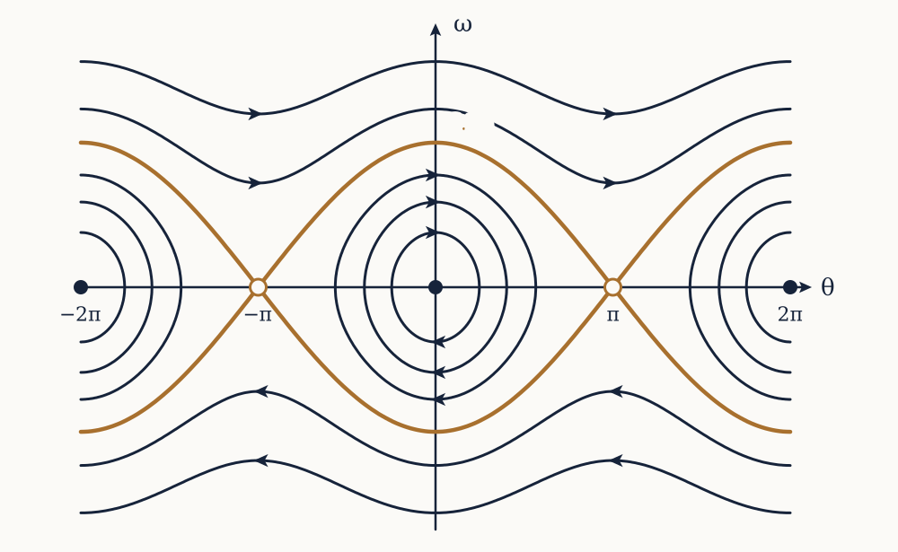
Example. A pendulum of length $1.00$ m hangs at rest. What angular speed at the bottom is just enough to carry it over the top, and what is its small-swing period?

The separatrix has the energy of the upright state at rest, $E = g / L$ . At the bottom, $E = {\frac{12}{ω}}^{2} - g / L$ , so ${\frac{12}{ω}}^{2} = 2 g / L$ and $ω_{c} = 2 \sqrt{g / L} = 2 \sqrt{9.81} = 6.26$ rad s⁻¹. At the bob that is a speed of $6.26$ m s⁻¹. The small-swing frequency is $\sqrt{9.81 / 1.00} = 3.13$ rad s⁻¹, giving a period of $2 π / 3.13 = 2.01$ s.

Now you. Do the same for a pendulum of length $0.50$ m.

Answer

$ω_{c} = 2 \sqrt{9.81 / 0.5} = 8.86$ rad s⁻¹, and the bob speed is $ω_{c} L = 4.43$ m s⁻¹. The small-swing frequency is $\sqrt{19.62} = 4.43$ rad s⁻¹, so the period is $1.42$ s, shorter by the square root of two as the length halved.

The price of the linear approximation

Isochronism, the amplitude-independent period that made pendulum clocks possible, is a property of the linearised equation only. Solving the exact equation by separating the energy relation gives the period as an elliptic integral, whose expansion in the amplitude $θ_{0}$ is

T = T_{0} (1 + \frac{θ_{0}^{2}}{16} + \frac{11 θ_{0}^{4}}{3072} + \dots)

with $θ_{0}$ in radians. The numbers say when to worry. At $10$ degrees the correction is $0.19$ per cent. At $30$ degrees it is $1.7$ per cent, which for a $1$ m pendulum means $2.041$ s against $2.006$ s, a clock losing twenty-five minutes a day if it were built wrong. At $90$ degrees the exact ratio is $1.180$ , and the two-term series gives $1.176$ , so even the correction needs correcting. As the amplitude approaches $180$ degrees the period diverges, which is the separatrix asserting itself: at $179$ degrees the true period is $3.90$ times the small-swing value, while the series predicts $1.95$ and is simply wrong.

This is the general shape of the relationship between a nonlinear system and its linearisation. The linear answer is exact in the limit, useful over a surprisingly wide range, and qualitatively false near the interesting boundary.

Predator and prey

Vito Volterra wrote the classic nonlinear system in 1926, prompted by a question from his son-in-law Umberto D'Ancona about fish catches. Let $x$ be prey and $y$ predators:

x' = a x - b x y, y' = - c y + d x y

Prey grow exponentially when alone and are eaten at a rate proportional to encounters, which is the product $x y$ ; predators starve when alone and breed in proportion to the same product. Every term is a modelling decision and the product terms are what make the system nonlinear.

There are two equilibria. At the origin, the linearisation has $f_{x} = a > 0$ and $g_{y} = - c < 0$ , so $Δ = - a c < 0$ : a saddle, and extinction of both is unstable, as it should be. The coexistence equilibrium is $x^{*} = c / d$ , $y^{*} = a / b$ , and there the partial derivatives are $f_{x} = 0$ , $f_{y} = - b x^{*} = - b c / d$ , $g_{x} = d y^{*} = d a / b$ , $g_{y} = 0$ . So $τ = 0$ and $Δ = a c > 0$ : a centre, with small oscillations of frequency $\sqrt{a c}$ .

Since it is a centre, the linearisation is inconclusive, and again a conserved quantity settles it. Dividing one equation by the other and separating gives

d x - c \ln x + b y - a \ln y = constant

whose level curves are closed loops around the equilibrium. So the oscillation is real, and predator and prey cycle indefinitely, the predator peak lagging the prey peak by a quarter of a cycle.

Example. Take $a = 0.6$ , $b = 0.02$ , $c = 0.4$ and $d = 0.01$ , in units of per year. Find the coexistence equilibrium and the period of small oscillations about it.

The equilibrium is $x^{*} = c / d = 40$ prey and $y^{*} = a / b = 30$ predators. The frequency is $\sqrt{a c} = \sqrt{0.24} = 0.490$ per year, so the period is $2 π / 0.490 = 12.8$ years. That is the right order for the famous lynx and hare records from the Hudson's Bay Company, which cycle at about ten years, though those data need a better model than this one.

Now you. Take $a = 0.8$ , $b = 0.04$ , $c = 0.5$ , $d = 0.02$ . Find the equilibrium and the period.

Answer

$x^{*} = 0.5 / 0.02 = 25$ and $y^{*} = 0.8 / 0.04 = 20$ . The frequency is $\sqrt{0.4} = 0.632$ per year, so the period is $9.9$ years.

Two results come out of this model that no amount of verbal reasoning would supply. The first is that the average of each population over one cycle equals its equilibrium value exactly, which follows from integrating $x' / x = a - b y$ over a period: the left side integrates to zero because $x$ returns to its starting value, so the average of $y$ is $a / b$ .

The second is Volterra's answer to D'Ancona. Harvest both species at rate $h$ , subtracting $h x$ and $h y$ : the equilibrium moves to $x^{*} = (c + h) / d$ and $y^{*} = (a - h) / b$ . Fishing therefore raises the average number of prey and lowers the average number of predators, and stopping fishing does the reverse. D'Ancona's records showed exactly that: the share of predatory fish in the catch at Fiume rose from about $12$ per cent before the First World War to $36$ per cent in 1918, when Adriatic fishing had almost stopped, and fell back to about $11$ per cent by 1923. The same logic warns that an insecticide killing both a pest and its predator can increase the pest's average population, which is a documented failure mode in agriculture.

The honest limit is severe. The centre depends on the model exactly as written. Add crowding among the prey, replacing $a x$ by the logistic $a x (1 - x / K)$ , and the centre becomes a stable spiral: the cycles damp out to a fixed point. Add a predation rate that saturates when prey are abundant, which is what real predators do, and the equilibrium can lose stability and throw off a stable cycle instead. Lotka-Volterra shows that predator-prey oscillation is possible without external forcing, and it is not evidence that any particular population cycles for that reason.

Limit cycles, and what a plane cannot do

The closed orbits above form a continuous family: each initial condition sits on its own loop, and a disturbance moves the system permanently to a neighbouring one. A real oscillator with a stable amplitude, such as a heartbeat or a clock escapement, does not behave that way: disturb it and the original amplitude comes back.

That requires a limit cycle, an isolated closed trajectory that nearby trajectories spiral onto. Van der Pol's equation, from his work on triode oscillators in the 1920s,

x'' - μ (1 - x^{2}) x' + x = 0

has one. Read the damping coefficient: $- μ (1 - x^{2})$ is negative for $| x | < 1$ , so small oscillations are pumped up, and positive for $| x | > 1$ , so large ones are damped. The system therefore settles onto one particular amplitude, near $2$ for small $μ$ , from any starting point except the origin. No linear system can do this, because scaling a solution of a linear system gives another solution, so amplitudes always come in continuous families.

There is also a strong negative result for the plane. The Poincaré-Bendixson theorem says that a trajectory of a two dimensional autonomous system that stays in a bounded region and does not approach an equilibrium must approach a closed orbit. So the plane permits equilibria and cycles and nothing more complicated. Everything wild needs at least three dimensions.

Where prediction ends

Three dimensions is where Edward Lorenz found the limit, in 1963, while truncating a convection model to three equations:

x' = σ (y - x), y' = x (ρ - z) - y, z' = x y - β z

With $σ = 10$ , $ρ = 28$ and $β = 8 / 3$ the trajectory is bounded, never repeats, and never settles: it winds around a set of zero volume, the attractor. Every equilibrium is unstable, so the classification of the previous lesson tells you where the solution cannot go and nothing about where it does.

The consequential property is sensitivity to initial conditions. Two trajectories starting a distance $ε$ apart separate roughly like $ε e^{λ t}$ , with $λ \approx 0.9$ per time unit for these parameters, so the gap doubles about every $0.77$ time units. Uniqueness still holds, and the system is entirely deterministic; what fails is usefulness, since the initial state is never known exactly. Improving the initial measurement by a factor of a thousand buys only about ten more doubling times of accurate forecast. That is why weather forecasts degrade over days rather than being extended indefinitely by better computers, and why forecasting moved to ensembles: run many slightly different initial states and report the spread, which is a statement about probability rather than about trajectory.

Chaos does not make the differential equation useless. The attractor's shape, the statistics of the motion, and the parameter values where behaviour changes character are all robust and computable. It changes what a solution is for.

What a solution says

That is the end of the subject, so it is worth naming what has been extracted from equations along the way, since almost none of it was a formula.

An equilibrium is a state the system can hold, and its stability says whether the world will let it. The eigenvalues there give the timescales: how long a disturbance takes to die, and whether it oscillates on the way. A conserved quantity constrains a whole trajectory without solving anything, which is how the pendulum's separatrix and the predator-prey loops were found. A bifurcation marks a parameter value where the qualitative answer changes, which is what made the harvested fishery collapse without warning. A frequency response says which inputs a system will amplify, which is what made the machine on its mounts shake and the bridge fail. And a Lyapunov exponent says how long a prediction is worth making.

The formulas of the first half of the course are the special cases where all of this collapses into an expression, and they are worth having for exactly that reason: a system you can solve is a system whose every question is already answered. For everything else, the equation still tells you what it does, provided you ask it the questions in this list rather than demanding $y (t)$ .