Autonomous equations and stability

An equation can be worth understanding even when its solution formula would be useless, and a large class can be understood without producing one at all.

The class is the autonomous equations, those of the form $y' = f (y)$ with no explicit $t$ on the right. The logistic equation is autonomous, Newton's cooling law is autonomous, a falling body with drag is autonomous. What they share is that the rule for how the system changes is the same at every instant: only the current state matters, which is what a law of nature usually looks like once the external drivers are absent.

That single property is enough to determine every solution's long-term behaviour from the graph of $f$ , with no integration.

Slopes that depend only on height

In the direction field of $y' = f (y)$ , the slope at a point depends on $y$ alone, so every horizontal line carries one slope repeated across the page. Two consequences follow immediately.

Solutions are translates of one another. If $y (t)$ solves the equation then so does $y (t - a)$ for any $a$ , because shifting the graph sideways does not change which height sits above which slope. So the whole family is one curve slid along the time axis, and the initial condition chooses the slide, not the shape.

Solutions are monotone. Between two consecutive roots of $f$ the sign of $f$ cannot change, since $f$ is continuous, so $y'$ keeps its sign and $y$ moves steadily one way. An autonomous first order equation cannot oscillate. That is a strong structural statement, and it is the reason this lesson ends by needing second order equations.

The phase line

Collapse the picture. Draw the $y$ axis alone, mark the roots of $f$ , and on each interval between them put an arrow pointing up where $f > 0$ and down where $f < 0$ . That is the phase line, and it contains everything about the long-run behaviour.

The roots are the equilibria, also called critical points or fixed points: if $f (y^{*}) = 0$ then the constant function $y \equiv y^{*}$ is a solution, and the system placed exactly there never moves. Every other solution moves along the arrow it starts on and either approaches the equilibrium at the far end or leaves towards infinity. It cannot pass an equilibrium, because that would require two solutions to cross at a point, which uniqueness forbids.

Three kinds of equilibrium exist. An equilibrium with arrows pointing towards it from both sides is stable, or a sink: small disturbances die. With arrows pointing away on both sides it is unstable, or a source: any disturbance grows. With one arrow in and one out it is semi-stable, attracting from one side and repelling on the other.

For the logistic equation $P' = r P (1 - P / K)$ the roots are $P = 0$ and $P = K$ . Between them $f > 0$ and above $K$ it is negative, so $0$ is unstable and $K$ is stable. That is the S-curve of the earlier lesson, read off in two lines instead of derived by partial fractions, and it also says what the formula did not make obvious: a population starting above $K$ falls to it, and no population ever crosses $K$ .

Example. Sketch the phase line for $y' = y^{2} - 4$ and describe the fate of solutions starting at $y = - 3$ , $y = 0$ and $y = 3$ .

The roots are $y = \pm 2$ . For $y < - 2$ , $f = y^{2} - 4 > 0$ , so the arrow points up. For $- 2 < y < 2$ it is negative, arrow down. For $y > 2$ it is positive again, arrow up. So $y = - 2$ has arrows pointing in from both sides and is stable, while $y = 2$ has arrows pointing away and is unstable. A solution from $y = - 3$ rises to $- 2$ . One from $y = 0$ falls to $- 2$ . One from $y = 3$ increases without bound, and in fact blows up in finite time, since the growth is quadratic.

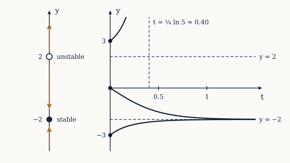
Now you. Do the same for $y' = y^{3} - y$ , classifying each of the three equilibria.

Answer

The roots are $y = - 1, 0, 1$ . The sign of $y (y - 1) (y + 1)$ is negative below $- 1$ , positive on $(- 1, 0)$ , negative on $(0, 1)$ and positive above $1$ . So the arrows point away from $- 1$ and away from $1$ , making both unstable, and towards $0$ from both sides, making it stable.

The linearisation test

Reading signs off a graph is reliable but slow, and there is a one-line test. Put $u = y - y^{*}$ , the displacement from an equilibrium, and expand $f$ in a Taylor series about $y^{*}$ . Since $f (y^{*}) = 0$ ,

u' = f (y^{*} + u) = f' (y^{*}) u + \frac{12}{f}'' (y^{*}) u^{2} + \dots

For small $u$ the first term dominates, so $u' \approx f' (y^{*}) u$ , whose solution is $u = u_{0} e^{f' (y^{*}) t}$ . The conclusion writes itself. If $f' (y^{*}) < 0$ the disturbance decays and the equilibrium is stable. If $f' (y^{*}) > 0$ it grows and the equilibrium is unstable. If $f' (y^{*}) = 0$ the linear term is absent and the test says nothing: $y' = y^{2}$ has a semi-stable equilibrium at zero, $y' = - y^{3}$ a stable one, $y' = y^{3}$ an unstable one, and all three have $f' = 0$ there.

The number $f' (y^{*})$ is more than a sign. Its reciprocal is the time constant of the approach: near a stable equilibrium the gap closes by a factor of $e$ every $1 / | f' (y^{*}) |$ units of time. For the logistic near $P = K$ , $f' (P) = r - 2 r P / K$ , so $f' (K) = - r$ and a population settles towards its capacity with time constant $1 / r$ , whatever the capacity is. With $r = 0.03$ per year that is $33$ years to close $63$ per cent of the gap and $\ln (10) / 0.03 = 77$ years to close $90$ per cent of it. Recovery is slow in a way the carrying capacity alone never tells you.

Terminal velocity read off the equation

A body falling with quadratic drag obeys $v' = g - \frac{b}{m} v^{2}$ , autonomous and nonlinear. The equilibrium is where drag balances weight, $v_{T} = \sqrt{m g / b}$ , and it is stable because $f' (v) = - 2 (b / m) v$ is negative there. No solving is needed to know that every skydiver approaches the same speed regardless of how they left the aircraft.

Example. A skydiver in a spread posture has $m / b = 300$ m. Find the terminal speed and the time constant of the approach to it.

The terminal speed is $\sqrt{300 \times 9.81} = 54.2$ m s⁻¹. The derivative there is $f' (v_{T}) = - 2 v_{T} / 300 = - 0.362$ s⁻¹, so the time constant is $1 / 0.362 = 2.8$ s. A useful way to remember it is $v_{T} / 2 g$ , which is the time gravity alone would take to reach half the terminal speed. The time constant describes the final approach rather than the whole fall: the exact solution from rest is $v = v_{T} \tanh (g t / v_{T})$ , which reaches $95$ per cent of terminal after $10.1$ s and about $350$ m, longer than three linearised time constants because early on the drag is far from balancing the weight.

Now you. In a head-down posture the same diver has $m / b = 800$ m. Find the terminal speed and the time constant.

Answer

$v_{T} = \sqrt{800 \times 9.81} = 88.6$ m s⁻¹, about $319$ km h⁻¹. The time constant is $v_{T} / 2 g = 88.6 / 19.62 = 4.5$ s, so the approach is slower as well as faster.

A landscape picture

Since $f$ depends on $y$ alone, define $V (y) = - \int f (y) d y$ , so that $y' = - V' (y)$ . Then along any solution

\frac{d V}{d t} = V' (y) y' = - {(y')}^{2} \leq 0

so $V$ never increases. The system slides downhill on the graph of $V$ and stops at the bottom of a valley. Stable equilibria are the minima of $V$ , unstable ones the maxima, and the depth of a valley says nothing about the rate: the curvature $V'' (y^{*}) = - f' (y^{*})$ does. This is the one dimensional case of the potential energy picture in mechanics, and it makes stability visual: a marble in a bowl returns, a marble on a dome does not.

A fishery that collapses without warning

Now put the theory to work on a model that is deliberately simple and still says something. Harvest a logistic population at a constant rate $H$ , meaning a fixed catch per year rather than a fixed effort:

\frac{d P}{d t} = r P (1 - \frac{P}{K}) - H

The equilibria solve a quadratic, and

P^{\pm} = \frac{K}{2} (1 \pm \sqrt{1 - \frac{4 H}{r K}})

Take $r = 0.4$ per year and $K = 1000$ tonnes. With $H = 80$ tonnes per year the square root is $\sqrt{0.2} = 0.447$ , giving equilibria at $724$ and $276$ tonnes. The upper one is stable, since $f' = r - 2 r P / K$ is $- 0.179$ there, and the lower is unstable, with $f' = + 0.179$ . So a stock above $276$ tonnes settles at $724$ and is fished indefinitely, and a stock below $276$ is driven to extinction by the harvest. There is a threshold, and it is not at zero.

Raise the catch and the two equilibria move towards each other. At $H = 90$ they are at $658$ and $342$ . At $H = r K / 4 = 100$ they meet at $P = K / 2 = 500$ , and above that the square root is imaginary: there are no equilibria at all, $P' < 0$ everywhere, and the population goes to zero from any starting size. The maximum sustainable catch is $r K / 4$ , exactly the peak growth rate found earlier.

Example. With $r = 0.4$ per year and $K = 1000$ tonnes, a fishery is harvested at $H = 90$ tonnes per year and the stock currently stands at $400$ tonnes. What happens, and what would happen at $500$ tonnes?

The equilibria are at $658$ and $342$ tonnes. A stock of $400$ lies between them, where $f > 0$ , so it grows to $658$ and stays. A stock of $500$ does the same. Both recover, but the margin above the unstable threshold is only $58$ tonnes in the first case, so a bad year could push the stock below $342$ , after which the same harvest drives it to zero.

Now you. The same fishery is harvested at $H = 96$ tonnes per year. Find the two equilibria, and say what happens to a stock of $400$ tonnes.

Answer

The square root is $\sqrt{1 - 384 / 400} = \sqrt{0.04} = 0.2$ , so the equilibria are at $500 (1 \pm 0.2)$ , that is $600$ and $400$ tonnes. A stock of exactly $400$ sits on the unstable equilibrium and stays there in principle, but any downward fluctuation sends it to zero.

Two features of this deserve naming. The first is that the collapse is not gradual. As $H$ rises from $90$ to $100$ the stable stock falls only from $658$ to $500$ , a modest decline that looks like a fishery under control, and then at $H = 100$ the stable state disappears entirely and the stock crashes. A qualitative change of this kind, where equilibria collide and annihilate as a parameter passes a critical value, is a bifurcation, and this one is the fold, the commonest of them all.

The second is that the safe margin shrinks as the catch rises: the unstable threshold climbs from $276$ to $342$ to $500$ while the stable state falls. A population sitting on a high yield is close to the boundary of its own basin of attraction, so ordinary environmental noise can push it across even before the bifurcation is reached. The Newfoundland cod fishery, closed by moratorium in 1992 after the northern stock fell to about one per cent of its historic biomass, is the standard illustration, and thirty years later the stock has not returned. The model does not explain that collapse, but it does explain why a fishery can look stable and be about to fail, which is more than a formula for $P (t)$ would have told anyone.

What one variable cannot do

Everything in this lesson rested on solutions being monotone, and that is also the limit. An autonomous first order equation cannot oscillate, cannot overshoot, and cannot return to a state it has left. Yet a plucked string, a swinging pendulum, an RLC circuit and a predator with its prey all do exactly those things.

The escape is to add a second dimension to the state. Position with velocity, or predator with prey, gives a plane to move in, and in a plane a trajectory can circle. Mechanics forces this on us anyway: Newton's second law involves acceleration, so the natural equation is second order. That is where the next lesson starts, and the theory has to be rebuilt for it, because an initial position no longer picks out a single solution.