Two problems algebra cannot solve

Two questions about a curve resist every technique in school mathematics, and calculus is the machinery built to answer them: how steep is a curve at one particular point, and how much area lies underneath it.

Both questions sound like geometry, and both are answered daily by anyone who reads a graph. What makes them hard is that the ordinary methods run out at exactly the moment they are needed. This lesson shows where they run out, what people did about it before the modern definitions existed, and why the two problems turn out to be the same problem twice. It assumes the algebra, functions and graphs of the previous course, plus the geometric series from its late lessons, and nothing else.

The slope of a curve at a point

A straight line has one slope, and it is the same everywhere on the line: pick any two points on it and the ratio of the rise to the run is the same number. That number is what the line means physically. Plot the position of a car against time, get a straight line, and its slope is the speed.

A curve has no such number. On the parabola $y = x^{2}$ the graph is nearly flat near the origin and steep at $x = 3$ , so any honest answer to "how steep is it" has to name a point. Ask for the steepness at exactly $x = 1$ and the difficulty appears immediately: slope is a ratio built from two points, and one point does not determine a ratio. Trying to compute the rise and run at a single point gives $0 / 0$ , which is not a number.

The obvious repair is to use a second point nearby and accept a small error. Take the point at $x = 1$ , where $y = 1$ , and a second at $x = 1 + h$ , where $y = (1 + h)^{2}$ . The line through the two, a secant, has slope

\frac{(1 + h)^{2} - 1}{h} = \frac{2 h + h^{2}}{h}

which for $h = 0.1$ is $2.1$ , for $h = 0.01$ is $2.01$ , and for $h = 0.001$ is $2.001$ . Coming in from the other side, $h = - 0.001$ gives $1.999$ . The numbers are converging on $2$ from both directions and never reaching it, and the one value of $h$ that would give the slope at the point itself, $h = 0$ , turns the fraction into $0 / 0$ and says nothing at all.

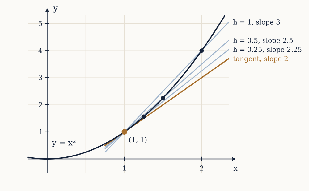
Something is clearly true here: the numbers are closing in on $2$ and would go on closing in forever. Saying what that means, precisely enough to calculate with, is the whole of the next lesson.

Example. Estimate the slope of $y = x^{3}$ at $x = 2$ using secants.

With $h = 0.1$ the second point is $x = 2.1$ , where $y = 9.261$ , so the secant slope is $(9.261 - 8) / 0.1 = 12.61$ . With $h = 0.01$ the point is $x = 2.01$ , where $y = 8.120601$ , giving $(8.120601 - 8) / 0.01 = 12.0601$ . With $h = 0.001$ the slope is $12.006001$ . The values are converging on $12$ , and every one of them is an honest slope of an honest line, none of which is the tangent.

Now you. Estimate the slope of $y = 1 / x$ at $x = 2$ with $h = 0.1$ , $h = 0.01$ and $h = 0.001$ .

Answer

The secant slope is $(1 / (2 + h) - 1 / 2) / h$ . For $h = 0.1$ that is $- 0.238095$ , for $h = 0.01$ it is $- 0.248756$ , and for $h = 0.001$ it is $- 0.249875$ . The values are closing on $- 0.25$ , and the sign is negative because the curve falls as $x$ increases.

The area under a curve

The second problem is older. Areas bounded by straight lines are elementary: a rectangle is a product, a triangle is half of one, and any polygon can be cut into triangles. Curved boundaries defeat this completely, because no finite number of straight cuts will follow a curve.

Take the region under $y = x^{2}$ from $x = 0$ to $x = 1$ . There is obviously an area there, somewhere between nothing and the unit square, but no formula in school geometry produces it. The available approximation is to fill the region with rectangles. Cut $[0, 1]$ into four strips of width $1 / 4$ and give each rectangle the height of the curve at the right end of its strip: the heights are $(1 / 4)^{2}, (2 / 4)^{2}, (3 / 4)^{2}, (4 / 4)^{2}$ , and the total area is $0.46875$ . Do the same with the left end of each strip and the total is $0.21875$ .

Those two numbers bracket the truth, because $x^{2}$ rises across the interval, so right ends overestimate and left ends underestimate. The bracket is embarrassingly wide. Going to ten strips narrows it to between $0.285$ and $0.385$ ; a hundred strips gives $0.32835$ to $0.33835$ ; a thousand gives $0.332834$ to $0.333834$ . The gap is closing on zero and both ends are closing on $1 / 3$ .

Again something is true and unstated. No finite number of rectangles ever gives the area, every one of them is wrong, and the sequence of wrong answers is unmistakably heading somewhere.

Example. Bracket the area under $y = x^{2}$ from $0$ to $1$ using five strips.

Each strip is $0.2$ wide. Right ends give heights $0.04, 0.16, 0.36, 0.64, 1$ , summing to $2.2$ , so the area estimate is $0.2 \times 2.2 = 0.44$ . Left ends give heights $0, 0.04, 0.16, 0.36, 0.64$ , summing to $1.2$ , for an estimate of $0.24$ . The true area lies between them, and the width of the bracket, $0.2$ , is exactly one strip width times the total rise of the function, which is a pattern worth remembering.

Now you. Bracket the area under $y = x^{2}$ from $0$ to $1$ using ten strips.

Answer

Each strip is $0.1$ wide. The right sum is $0.1 \times (0.01 + 0.04 + \dots + 1.00) = 0.385$ and the left sum is $0.285$ . The bracket has halved in width, as expected, and still contains $1 / 3$ .

What Archimedes did about it

The area problem was solved, in particular cases, about nineteen centuries before calculus existed. Archimedes of Syracuse, working around 240 BC, computed the exact area of a parabolic segment: the region cut off from a parabola by a straight chord.

His construction inscribes the largest triangle in the segment, then the two largest triangles in the two gaps that remain, then four in the four gaps left by those, and so on. He proved geometrically that each generation of triangles has one quarter of the total area of the previous generation. The segment is therefore the first triangle multiplied by $1 + 1 / 4 + 1 / 16 + 1 / 64 + \dots$ , and that geometric series sums to $4 / 3$ . The area of the segment is four thirds of the inscribed triangle, exactly, with no approximation surviving in the answer.

The same author bracketed $π$ in Measurement of a Circle by inscribing and circumscribing regular polygons of $96$ sides, obtaining $3 \frac{10}{71} < π < 3 \frac{1}{7}$ , which is $3.14085 < π < 3.14286$ , against the true $3.14159$ . The technique, called the method of exhaustion, is rigorous by any standard: to prove the area equals $A$ , show that assuming it larger and assuming it smaller both lead to contradictions.

The trouble with exhaustion is that it is a proof technique, not a method of discovery. Each new region needs its own geometric argument, invented from nothing, and Archimedes needed to know the answer before he could prove it. Two thousand years produced only a handful of successes. What was missing was not rigour but a procedure.

The two problems are one

Here is the connection that makes a subject out of two puzzles, and it is easiest to see in physics. Let $s (t)$ be the distance a body has travelled by time $t$ , and $v (t)$ its speed. If you plot $s$ against $t$ , the slope at any instant is the speed at that instant: speed is a rate, and a rate is a slope. If instead you plot $v$ against $t$ , the area under the graph up to time $t$ is the distance covered, since distance is speed accumulated over time.

So the slope problem takes position to speed, and the area problem takes speed back to position. They run in opposite directions between the same two quantities, which suggests they are inverse operations, and that whichever is easier to compute solves both.

A falling body makes the claim checkable. Near the Earth's surface a body released from rest falls with speed $v = 9.8 t$ metres per second after $t$ seconds, which plots as a straight line through the origin. The area under it from $0$ to $3$ seconds is a triangle of base $3$ and height $29.4$ , so the area is $44.1$ . The distance formula for constant acceleration, from mechanics, is $s = \frac{12}{g} t^{2}$ , giving $\frac{12}{(} 9.8) (9) = 44.1$ metres. The area under the speed graph is the distance, to the last digit.

Example. Use the area under $v = 9.8 t$ to find the distance fallen in $5$ seconds, and check it.

The region is a triangle of base $5$ and height $9.8 \times 5 = 49$ , so the area is $\frac{12}{(} 5) (49) = 122.5$ . The formula $s = \frac{12}{g} t^{2}$ gives $\frac{12}{(} 9.8) (25) = 122.5$ metres. They agree, and notice that the area calculation needed no formula for falling bodies: it read the answer off the graph.

Now you. A car accelerates from rest so that its speed is $v = 4 t$ metres per second. How far does it travel in the first $6$ seconds, and what is the slope of the distance graph at $t = 6$ ?

Answer

The area under $v = 4 t$ from $0$ to $6$ is a triangle of base $6$ and height $24$ , so the distance is $72$ metres. The slope of the distance graph at $t = 6$ is the speed there, which is $4 \times 6 = 24$ metres per second. The two problems are answering each other.

Ghosts of departed quantities

Isaac Newton and Gottfried Wilhelm Leibniz, working independently in the 1660s and 1670s, each found the procedure that exhaustion lacked, and each published a calculus in which slopes and areas are computed by rules rather than reinvented per problem. Newton spoke of fluxions, rates at which quantities flow; Leibniz wrote $d x$ and $d y$ for infinitesimal differences and invented the notation still used today. The results were spectacular and immediately convincing, because they reproduced everything the ancients had done and much they had not.

The reasoning was not defensible. In a typical Leibnizian calculation, $d x$ is a quantity small enough that $(d x)^{2}$ may be discarded as negligible, and at the end of the calculation $d x$ is divided out, which requires it to be non-zero, and then dropped, which requires it to be zero. Bishop George Berkeley attacked exactly this in The Analyst of 1734, asking of the vanishing increments: "May we not call them the ghosts of departed quantities?" The complaint was fair, and no clean answer existed for almost a century.

The repair came from Augustin-Louis Cauchy, whose Cours d'Analyse of 1821 made the limit rather than the infinitesimal the basic notion, and from Karl Weierstrass, who in the 1860s gave the limit the tolerance-based definition that removes every appeal to intuition about the infinitely small. Nothing in the results changed. What changed is that the results acquired proofs.

Two remarks about that history are worth carrying forward. First, useful mathematics is regularly used for a century before it is made rigorous, so a working physicist's cheerful manipulation of $d x$ is not ignorance but inheritance. Second, the rigorous version is not decoration: without it there is no way to tell a valid infinitesimal argument from an invalid one, and both kinds were published.

What the rest of this course does

The plan follows the trouble. The immediate need is a precise account of what it means for the secant slopes to close in on $2$ , which is the limit, and that occupies the next two lessons, since the limit also settles what it means for a function to have no breaks in it.

With limits available, the slope problem is solved in one definition and then made practical: a handful of rules reduce a page of limit algebra to a line, and by the middle of the course any function that can be written down can be differentiated. Those derivatives immediately answer questions that look nothing like slopes, from the maximum range of a projectile to the angle at which light bends entering water.

The area problem is then defined properly as a limit of rectangle sums, computed the hard way once, and after that the connection glimpsed above is proved as the Fundamental Theorem of Calculus. That theorem converts every area problem into the search for a function with a given derivative, which is what makes areas, volumes, work and averages computable at all.

The last lesson does the reverse trick: instead of computing exactly, it replaces a function by a polynomial that matches it near a point, which is where every approximation in a physics textbook comes from. Before any of that, a definition is owed.