The Fundamental Theorem

The area under a curve has been defined as a limit of sums, and computing even the simplest case took a closed form for the sum of squares, so the definition needs to be rescued by a theorem.

The rescue is the result that gives this course its shape: the two problems of the first lesson, the slope and the area, are inverse operations. Everything needed for the proof is already available, namely the Mean Value Theorem for integrals from the previous lesson and the corollary from the lesson before it that two functions with the same derivative differ by a constant.

The area so far

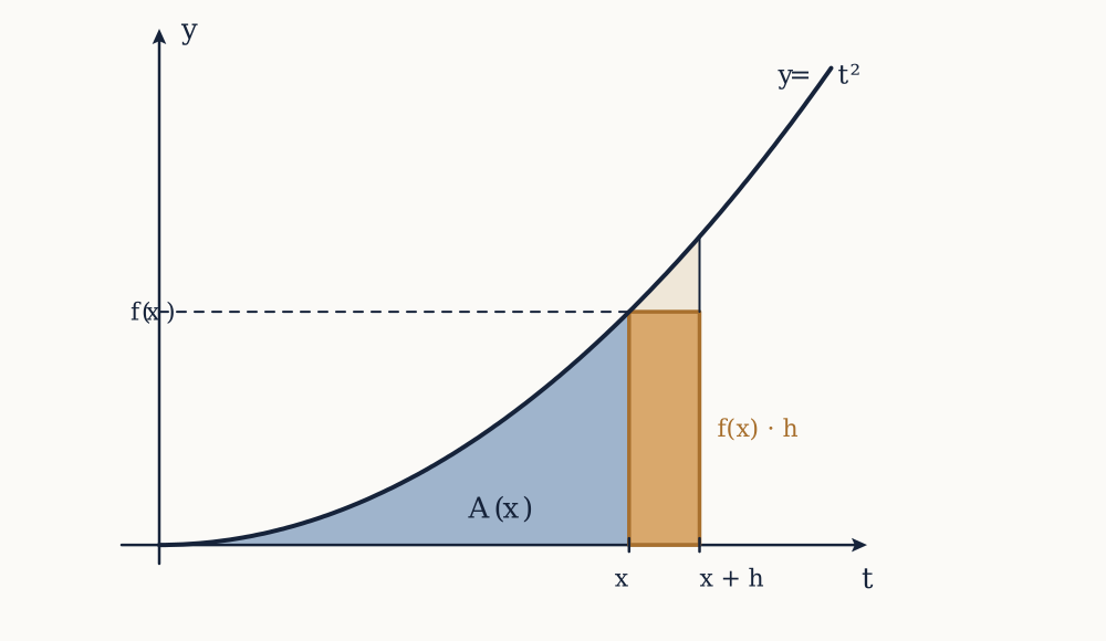
Fix a function $f$ , continuous on $[a, b]$ , and define a new function by letting the upper limit vary:

A (x) = \int_{a}^{x} f (t) d t

This is the area accumulated from the fixed left end $a$ up to the movable point $x$ . The variable of integration is written $t$ rather than $x$ deliberately, because $x$ is now doing a different job as the endpoint; using the same letter for both is a common source of confusion and no more than that, since the variable of integration means nothing outside the integral.

$A$ is a perfectly ordinary function. For $f (t) = t^{2}$ and $a = 0$ , the calculation of the previous lesson generalises to give $A (x) = x^{3} / 3$ : the same Riemann sum with $x$ in place of $1$ produces $x^{3}$ times the same limit. Differentiate that and you get $x^{2}$ , which is $f$ again. That is not a coincidence, and it is not special to this function.

The first half

Fundamental Theorem, part one. If $f$ is continuous on $[a, b]$ , then $A$ is differentiable and $A^{'} (x) = f (x)$ for every $x$ in the interval.

The proof takes four lines. The difference $A (x + h) - A (x)$ is $\int_{a}^{x + h} f - \int_{a}^{x} f$ , which by additivity is $\int_{x}^{x + h} f$ : the area of the thin sliver between $x$ and $x + h$ . So the difference quotient is

\frac{A (x + h) - A (x)}{h} = \frac{1}{h} \int_{x}^{x + h} f (t) d t

and the right side is exactly the average value of $f$ over the sliver. By the Mean Value Theorem for integrals there is a point $c$ between $x$ and $x + h$ where $f (c)$ equals that average. As $h \to 0$ the point $c$ is squeezed toward $x$ , and since $f$ is continuous, $f (c) \to f (x)$ . Therefore $A^{'} (x) = f (x)$ .

Read as a sentence, it says the rate at which area accumulates is the height of the curve, which is obvious once heard: widen the region by a sliver of width $h$ and you gain about $f (x) \cdot h$ of area. Continuity is what makes "about" into "exactly in the limit".

The immediate consequence is an existence theorem that nothing else supplies: every continuous function has an antiderivative, namely its own area function. Whether that antiderivative can be written in terms of familiar functions is a separate question, and often the answer is no.

The second half

Fundamental Theorem, part two. If $f$ is continuous on $[a, b]$ and $F$ is any function with $F^{'} = f$ there, then

\int_{a}^{b} f (x) d x = F (b) - F (a)

The proof is where the Mean Value Theorem pays for itself. By part one, $A$ is an antiderivative of $f$ . So $F$ and $A$ have the same derivative on the interval, and by the corollary proved two lessons ago they differ by a constant: $F (x) = A (x) + C$ . Now evaluate at both ends and subtract. Since $A (a) = 0$ , we get $F (b) - F (a) = A (b) - A (a) = A (b)$ , which is $\int_{a}^{b} f$ .

The word any in the statement is what the corollary buys. There are infinitely many antiderivatives, differing by a constant, and every one of them gives the same answer because the constant cancels in the subtraction. Without the theorem that they differ only by a constant, there would be no reason to expect that.

A function with $F^{'} = f$ is called an antiderivative of $f$ , and the whole family is written with the indefinite integral sign,

\int f (x) d x = F (x) + C

The $C$ is not decoration. Omitting it makes no difference in a definite integral, and it is the entire content of the answer in a differential equation, where the constant is fixed by an initial condition.

What this actually means

Two problems that look unrelated, the slope of a curve and the area under one, have turned out to be inverse operations. Differentiating an area function returns the integrand; integrating a derivative returns the original function up to a constant.

That is the discovery Newton and Leibniz are credited with, and it is worth being precise about the credit. Tangents had been drawn by Fermat and Descartes, and areas computed by Cavalieri, Wallis and others, before either of them was born. What neither predecessor had was the theorem connecting the two, which converts an intractable limit of sums into a search for an antiderivative, and it is the connection that turned a collection of clever special cases into a subject with an algorithm.

Practically, the theorem hands over a table of integrals for free: every differentiation rule, read backwards, is an antiderivative. From the power rule, $\int x^{n} d x = x^{n + 1} / (n + 1) + C$ for every $n$ except $- 1$ , where the formula would divide by zero and where the answer is instead $\ln | x | + C$ , the gap in the power rule noticed in the transcendental lesson. From the trigonometric derivatives, $\int \sin x d x = - \cos x + C$ and $\int \cos x d x = \sin x + C$ . From the exponential, $\int e^{x} d x = e^{x} + C$ . From the inverse functions, $\int d x / (1 + x^{2}) = \arctan x + C$ and $\int d x / \sqrt{1 - x^{2}} = \arcsin x + C$ .

Example. Evaluate $\int_{0}^{π} \sin x d x$ and $\int_{1}^{2} \frac{d x}{x}$ .

An antiderivative of $\sin x$ is $- \cos x$ , so the first integral is $[- \cos x]$ evaluated from $0$ to $π$ , which is $- \cos π + \cos 0 = 1 + 1 = 2$ . An antiderivative of $1 / x$ is $\ln x$ , positive throughout $[1, 2]$ , so the second is $\ln 2 - \ln 1 = 0.693147$ . Compare that with the previous lesson, where four midpoint rectangles gave $0.691220$ after a paragraph of arithmetic: the theorem produces a better answer in one line.

Now you. Evaluate $\int_{0}^{2} (3 x^{2} - 2 x) d x$ .

Answer

An antiderivative is $x^{3} - x^{2}$ , so the value is $(8 - 4) - (0 - 0) = 4$ .

Net change

Part two, read in the other direction, is the statement that most applications actually use. If $F$ is any quantity and $F^{'}$ its rate of change, then

\int_{a}^{b} F^{'} (t) d t = F (b) - F (a)

the total change in the quantity over the interval. Integrating a rate recovers the amount. That single sentence covers a velocity integrating to a displacement, a flow rate integrating to a volume, a power integrating to an energy, a current integrating to a charge, and a marginal cost integrating to a total cost.

Example. Water flows into a tank at $r (t) = 200 + 20 t$ litres per minute. How much enters during the first ten minutes?

The amount is $\int_{0}^{10} (200 + 20 t) d t$ . An antiderivative is $200 t + 10 t^{2}$ , so the value is $2000 + 1000 = 3000$ litres. The check is available because the rate is linear: it runs from $200$ to $400$ litres per minute, averaging $300$ , and $300 \times 10 = 3000$ .

Now you. A particle has velocity $v (t) = t^{2} - 4$ metres per second. Find its displacement over the first three seconds, and the distance it travels.

Answer

The antiderivative is $t^{3} / 3 - 4 t$ , so the displacement is $(9 - 12) - 0 = - 3$ metres: it ends up three metres behind where it started. For the distance, note that $v < 0$ until $t = 2$ and positive after. Over the first stretch the position falls by $5.333$ metres, and the second contributes $- 3 - (- 5.333) = 2.333$ metres, so the distance travelled is $7.667$ metres.

Where part two goes wrong

The hypothesis that $f$ is continuous on the whole interval is not a formality, and skipping it produces answers that are visibly absurd.

Consider $\int_{- 1}^{1} \frac{d x}{x^{2}}$ . An antiderivative of $x^{- 2}$ is $- x^{- 1}$ , and evaluating gives $- 1 - (+ 1) = - 2$ . That is impossible: the integrand is positive everywhere it is defined, so any sensible notion of area cannot be negative. The error is that the integrand is unbounded at $x = 0$ , which is inside the interval, so it is not continuous there and the theorem does not apply. The integral is in fact divergent, in the sense made precise in a later lesson.

The lesson generalises. Before quoting an antiderivative across an interval, check that both the function and the antiderivative behave throughout it. Integrands with a vertical asymptote inside the range, and antiderivatives such as $\tan x$ that jump at a point of the range, are where confident nonsense comes from.

Part one with a chain rule

Part one is used less often for computing and more often for differentiating a function that is defined as an integral, which happens whenever an antiderivative cannot be written down.

If the upper limit is a function of $x$ rather than $x$ itself, the chain rule applies. Writing $G (x) = \int_{a}^{u (x)} f (t) d t$ as a composition of the area function with $u$ , part one gives $A^{'} = f$ and so

G^{'} (x) = f (u (x)) \cdot u^{'} (x)

Example. Differentiate $G (x) = \int_{1}^{x^{3}} \ln t d t$ and evaluate at $x = 2$ .

Here $f (t) = \ln t$ and $u = x^{3}$ , so $G^{'} (x) = \ln (x^{3}) \cdot 3 x^{2} = 9 x^{2} \ln x$ . At $x = 2$ that is $36 \ln 2 = 24.953$ . No antiderivative of $\ln t$ was needed, and none was used.

Now you. Differentiate $G (x) = \int_{0}^{x^{2}} \sqrt{1 + t} d t$ and evaluate at $x = 2$ .

Answer

With $u = x^{2}$ , the rule gives $G^{'} (x) = \sqrt{1 + x^{2}} \cdot 2 x$ , which at $x = 2$ is $4 \sqrt{5} = 8.944$ .

Functions defined this way are not exotic. The error function of statistics is $\erf (x)$ , defined as a multiple of $\int_{0}^{x} e^{- t^{2}} d t$ , and the sine integral of optics is $\int_{0}^{x} (\sin t) / t d t$ . Neither integrand has an antiderivative expressible in elementary terms, so the integral is the definition, and part one is what says these functions are differentiable and gives their derivatives.

The new difficulty

The theorem has moved the problem rather than removing it. Every definite integral is now as easy as recognising the integrand as somebody's derivative, and that recognition is the hard part.

Differentiation is an algorithm: apply the rules from the outside in and an answer always comes out. Antidifferentiation is a search. There is no rule that inverts the product rule directly, no rule that inverts the chain rule directly, and no procedure guaranteed to terminate. What exists instead is a set of techniques that convert unfamiliar integrands into familiar ones, and a large body of integrals that no technique will ever crack because their antiderivatives are not elementary functions at all.

The next lesson covers the techniques, and is honest about where they stop.