Functions of several variables

The pressure of a gas depends on its volume and on its temperature at the same time, and the calculus of one variable, built for a quantity that depends on a single number, has no way to ask how that pressure changes when both are free to move.

The previous course was about $y = f (x)$ : one input, one output, a curve with one slope at each point. Almost nothing measured in a laboratory, a factory or a weather station behaves like that. This lesson sets up the objects the rest of this course differentiates and integrates, shows three ways of looking at them, and ends on the precise reason the old machinery breaks. It assumes Calculus I and nothing about vectors or three dimensional geometry.

One output, several inputs

A function of two variables is a rule that takes an ordered pair of real numbers $(x, y)$ and returns one real number, written $f (x, y)$ . The pair is best thought of as a single input, a point in the plane, because the question will always be what happens as the point moves. A function of three variables takes a point $(x, y, z)$ , and so on.

The ideal gas law is the standard example. For $n$ moles of gas at absolute temperature $T$ in a volume $V$ , the pressure is

p (V, T) = \frac{n R T}{V}

with $R = 8.314$ joules per mole per kelvin. One mole at the freezing point of water, $T = 273.15$ K, in a volume of $0.0224$ cubic metres, has $p = 8.314 \times 273.15 / 0.0224 = 101 383$ Pa, which is within a tenth of a percent of the standard atmosphere of $101 325$ Pa.

Economics has the same shape. In 1928 the mathematician Charles Cobb and the economist Paul Douglas fitted index numbers for American manufacturing from 1899 to 1922, labour $L$ and capital $K$ , to a production function of the form

Q (L, K) = 1.01 L^{3 / 4} K^{1 / 4}

and found that it tracked the actual output index closely for all twenty four years. The exponents add to $1$ , which has a checkable meaning: doubling both inputs gives $1.01 (2 L)^{3 / 4} (2 K)^{1 / 4} = 2^{3 / 4 + 1 / 4} Q = 2 Q$ , so doubling the factory doubles its output.

Weather forecasts supply a third. Since November 2001 the weather services of Canada and the United States have reported a wind chill index computed from the air temperature $T$ in degrees Celsius and the wind speed $v$ in kilometres per hour measured at ten metres:

W (T, v) = 13.12 + 0.6215 T - 11.37 v^{0.16} + 0.3965 T v^{0.16}

The output is the temperature which, in near-calm air, would draw heat from exposed skin at the same rate. It is a fitted model of heat loss from a human face, not a law of nature.

Example. Find the wind chill at $T = - 5$ with a wind of $v = 30$ .

First $30^{0.16} = 1.7232$ . Then the four terms are $13.12$ , $0.6215 \times (- 5) = - 3.1075$ , $- 11.37 \times 1.7232 = - 19.593$ and $0.3965 \times (- 5) \times 1.7232 = - 3.4163$ . Their sum is $W = - 13.0$ . A thermometer reading of $- 5$ °C in a 30 km/h wind feels like $- 13$ °C.

Now you. Find the wind chill at $T = - 10$ with $v = 20$ , to one decimal place.

Answer

Here $20^{0.16} = 1.6150$ , and the terms are $13.12$ , $- 6.215$ , $- 18.362$ and $- 6.403$ , which sum to $W = - 17.9$ . The air is $5$ degrees colder than in the example and the wind is lighter, and the second effect recovers only a little of the first.

Where a function is defined

A function of two variables is defined on a set of points in the plane, its domain, and domains in the plane come in far more shapes than intervals on a line.

When a formula is given without comment, the domain is taken to be every point where the formula makes sense. For $f (x, y) = \sqrt{9 - x^{2} - y^{2}}$ the square root needs $x^{2} + y^{2} \leq 9$ , and since $x^{2} + y^{2}$ is the square of the distance from the origin, the domain is the disc of radius $3$ centred there, boundary circle included. For $g (x, y) = \ln (x - y)$ the logarithm needs $x - y > 0$ , which is every point strictly below the line $y = x$ : a half-plane, with its edge excluded. And $h (x, y) = x y / (x^{2} + y^{2})$ is defined everywhere except the single point $(0, 0)$ , a hole of a kind that has no counterpart on the real line, because a point in the plane can be approached from every direction at once. A later lesson shows that this particular hole cannot be filled.

Physical models add restrictions the algebra does not see. The gas law makes sense only for $V > 0$ and $T > 0$ , but it is also only accurate where the gas is dilute: squeeze carbon dioxide hard enough at room temperature and it liquefies, while the formula carries on regardless. The wind chill formula is published with the conditions $T \leq 10$ and $v \geq 4.8$ attached, because outside them the underlying experiment says nothing. The honest domain of a model is where it was tested.

Graphs are surfaces

The graph of $y = f (x)$ needs two axes, one for the input and one for the output. A function of two variables needs three. Its graph is the set of points $(x, y, z)$ with $z = f (x, y)$ , drawn with the $x$ and $y$ axes flat on a table and the $z$ axis pointing up, so that above each point of the domain there is exactly one point of the graph, at height $f (x, y)$ . Those points form a surface, lying over the domain the way a landscape lies over a map.

Take $f (x, y) = x^{2} + y^{2}$ . The height at each point is its squared distance from the origin, so all points at distance $r$ sit at height $r^{2}$ . The surface is a bowl called a paraboloid, flat at the bottom and steepening outwards. Take instead $f (x, y) = \sqrt{9 - x^{2} - y^{2}}$ , defined on the disc of radius $3$ . Squaring $z = \sqrt{9 - x^{2} - y^{2}}$ gives $x^{2} + y^{2} + z^{2} = 9$ , which says every point of the graph is at distance $3$ from the origin in space, and since $z \geq 0$ the graph is the upper half of a sphere, a dome sitting on its domain.

The most useful trick for handling a surface is to slice it. Fixing $y = b$ cuts the surface with a vertical plane, and what remains is the curve $z = f (x, b)$ , an ordinary function of the single variable $x$ called a trace. The paraboloid sliced at $y = 2$ gives $z = x^{2} + 4$ , a parabola lifted by $4$ . The dome sliced at $y = 0$ gives $z = \sqrt{9 - x^{2}}$ , a semicircle. Every trace is a problem from the previous course.

The wind chill surface shows how different the traces in two directions can be. Hold the wind at $v = 30$ and the formula collapses to $W = - 6.473 + 1.3048 T$ : a straight line, saying that in that wind every degree of real cooling feels like $1.3$ degrees. Hold the temperature at $- 5$ instead and $W = 10.0125 - 13.3525 v^{0.16}$ , a curve that falls steeply for light winds and flattens for strong ones, since going from $10$ to $20$ km/h costs $2.3$ degrees of wind chill and going from $40$ to $50$ costs only $0.9$ . One surface, straight when walked one way and bent when walked the other.

Level curves

The second way of looking at a surface slices it horizontally instead. The level curve of $f$ at height $c$ is the set of points in the domain where $f (x, y) = c$ : cut the surface at height $c$ and drop the cut onto the input plane. Drawing several level curves for equally spaced values of $c$ , each labelled with its value, gives a picture of the whole function using only two dimensions.

For the paraboloid the level curve $x^{2} + y^{2} = c$ is a circle of radius $\sqrt{c}$ . At $c = 1, 2, 3, 4$ the radii are $1$ , $1.414$ , $1.732$ and $2$ , so the circles crowd together further out. That crowding is the steepening of the bowl: the height rises by the same step between each pair of circles, and it does so over shorter and shorter distances.

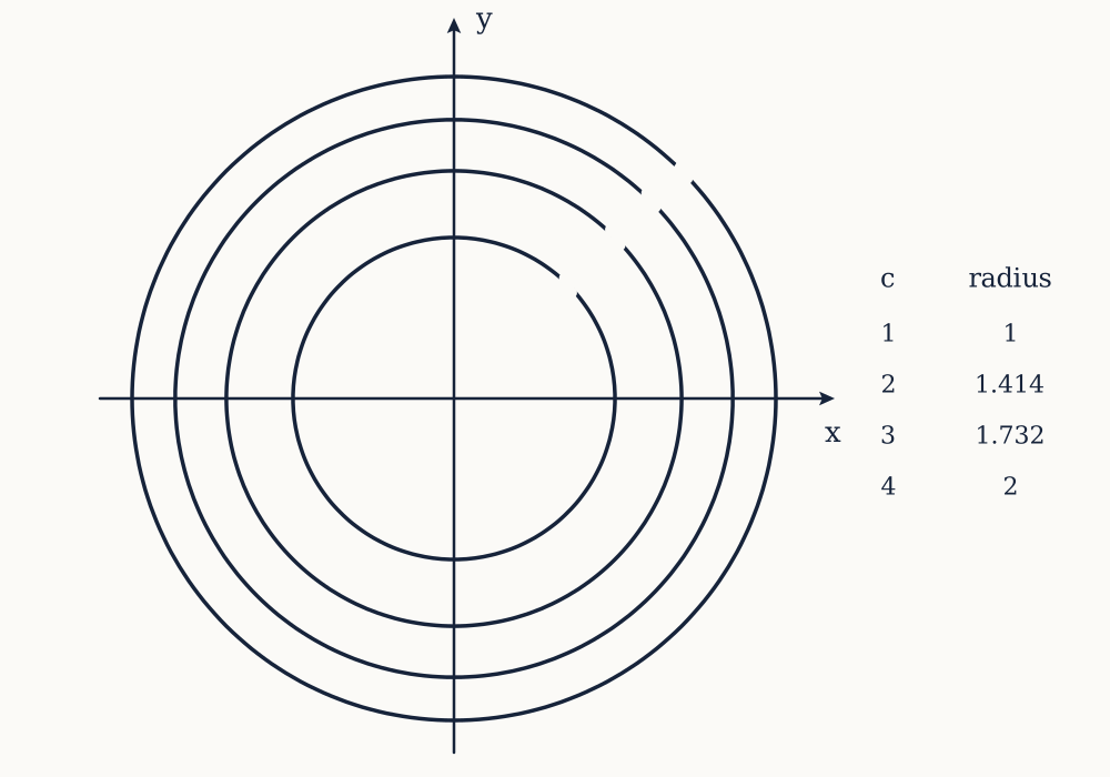
Level curves of x² + y² at c = 1, 2, 3 and 4: circles of radius 1, 1.414, 1.732 and 2. Each step in c is the same, but the circles get closer together further out, where the bowl is steeper.

Level curves have been reinvented in every subject that needed them. Temperature as a function of volume and pressure, $T = p V / (n R)$ , has level curves $p V = constant$ , the hyperbolas Robert Boyle measured in 1662 and physicists still call isotherms. Meteorologists draw isobars of equal pressure. Economists draw isoquants, the combinations of labour and capital giving equal output. Cartographers draw contours. The mathematics is the same in every case: a curve along which the function does not change.

For the Cobb-Douglas function the isoquant at output $Q_{0}$ can be solved explicitly. Write $c = Q_{0} / 1.01$ , so that $L^{3 / 4} K^{1 / 4} = c$ , and raise both sides to the fourth power to get $L^{3} K = c^{4}$ , that is $K = c^{4} / L^{3}$ . Along an isoquant, capital must rise as the cube of the fall in labour.

Example. A plant with Cobb-Douglas production $Q = 1.01 L^{3 / 4} K^{1 / 4}$ runs at $L = 16$ , $K = 81$ . If labour is halved, how much capital keeps output the same?

The current output is $1.01 \times 16^{3 / 4} \times 81^{1 / 4} = 1.01 \times 8 \times 3 = 24.24$ , so $c = 24$ and the isoquant is $K = 24^{4} / L^{3} = 331 776 / L^{3}$ . At $L = 8$ that is $331 776 / 512 = 648$ . Halving labour needs eight times the capital, the factor $2^{3}$ that $K = c^{4} / L^{3}$ predicts without computing $c$ at all.

Now you. The same plant runs at $L = 81$ , $K = 16$ . If labour is cut to $27$ , how much capital keeps output the same?

Answer

Now $c = 81^{3 / 4} \times 16^{1 / 4} = 27 \times 2 = 54$ , and the isoquant is $K = 54^{4} / L^{3}$ . At $L = 27$ this gives $K = 8 503 056 / 19 683 = 432$ . Labour fell by a factor of $3$ , so capital rose by $3^{3} = 27$ , from $16$ to $432$ .

Reading a contour map

Contour lines on maps have a mathematical origin. Charles Hutton, reducing the survey of the Scottish mountain Schiehallion made for Nevil Maskelyne's 1774 experiment to weigh the Earth, needed the volume of the mountain and had a mass of spot heights to organise; joining points of equal height turned the numbers into a picture, and his report of 1778 is often credited with the first contours of land relief. A walker's map is a level-curve diagram of height above sea level.

The Ordnance Survey's 1:50,000 Landranger maps of Great Britain draw contours every $10$ metres, and at that scale one millimetre on the paper is $50$ metres on the ground. Count the contour gaps crossed along a route to get the rise, measure the route on the map to get the run, and divide. Closely packed contours mean a steep slope, widely spaced ones a gentle slope, and walking along a contour means not climbing at all.

Example. On a Landranger map a path crosses five contour gaps in $4$ mm of paper. What is its average gradient, and at what angle does it climb?

The rise is $5 \times 10 = 50$ metres and the run is $4 \times 50 = 200$ metres, so the gradient is $50 / 200 = 0.25$ , a slope of one in four. The angle is $\arctan 0.25 = 14.0$ degrees.

Now you. A route crosses eight contour gaps in $5$ mm on the same map. Find the gradient and the angle.

Answer

The rise is $80$ metres and the run is $250$ metres, so the gradient is $0.32$ and the angle is $\arctan 0.32 = 17.7$ degrees.

Why one variable is not enough

The contour map already says what goes wrong. On a hillside the steepness depends on which way you walk: straight up the fall line it is greatest, along the contour it is zero, and every compass bearing in between gives something else. A function of one variable has one line through each point to move along; a function of two variables has a slope in every direction.

The paraboloid $f (x, y) = x^{2} + y^{2}$ at the point $(3, 4)$ , where $f = 25$ , makes this quantitative. Step a distance $0.001$ due east, to $(3.001, 4)$ , and the difference quotient is $6.001$ . Step due north instead and it is $8.001$ . Step directly away from the origin, $0.0006$ east and $0.0008$ north, and it is $10.001$ . Step along the level circle through the point, $0.0008$ west and $0.0006$ north, and it is $0.001$ , heading for zero. Four directions, four limits, $6$ , $8$ , $10$ and $0$ , and there are infinitely many more.

The same thing happens with the gas. At $T = 273.15$ K and $V = 0.0224$ cubic metres, warming one mole by a kelvin raises the pressure by $371$ Pa, while adding a litre of volume lowers it by $4 333$ Pa. Doing both at once lowers it by $3 977$ Pa, close to the sum of the two separate changes, a hint that the separate rates may be enough to recover the rest.

So the derivative of the previous course cannot be reused as it stands. Its difference quotient divided a change in output by a change in input, and here the input change is a step in the plane with both a length and a direction. The limit is affected too: at the hole in $x y / (x^{2} + y^{2})$ the origin can be approached along infinitely many lines and curves, not just from the left and from the right. And the graph is a surface, so whatever replaces the tangent line must be a plane.

Every one of those needs geometry the previous course never built: distance between points in space, directions described by numbers, and equations for planes. That is the work of the next lesson, which sets up vectors in three dimensions.