Every structure so far holds a collection of items whose only relationship is the order of their keys, and a great deal of real data is not shaped like that.
Roads join towns, functions call functions, packages depend on packages, web pages link to web pages, people know people. In all of these the relationships are the data, and the questions asked are about them: is there a route, what is the shortest one, is anything circular, what must be built before what. None of those questions can even be stated in terms of an array, a hash table or a tree. They need an object whose whole content is which things connect to which.
Vertices and edges
A graph is a set of vertices and a set of edges, each edge joining a pair of vertices. That is the entire definition, and its generality is the point: a tree is a graph, a linked list is a graph, a road map is a graph.
Three choices specialise it. Edges may be undirected, so an edge between and can be traversed either way, as with a friendship or a two-way street; or directed, an arrow from to only, as with a one-way street, a function call or a package dependency. Edges may be unweighted, when only their existence matters, or weighted, when each carries a number: a distance, a cost, a capacity, a duration. And the graph may or may not allow self-loops and repeated edges, which most applications do not.
The vocabulary is worth fixing because the algorithms are stated in it. The degree of a vertex is the number of edges at it, split into in-degree and out-degree when directed. A path is a sequence of vertices each joined to the next; a cycle is a path returning to its start. A graph is connected if a path joins every pair, and a directed graph is strongly connected if that holds respecting the arrows. A directed graph with no cycles is a DAG, a directed acyclic graph, which is the shape of every dependency system.
Two size facts govern everything below. An undirected graph on vertices has at most edges, so . A graph is called sparse when is closer to and dense when it approaches , and nearly every large real graph is sparse: road networks have an average degree near 3, because junctions have three or four roads, and social networks have an average degree in the hundreds against billions of users.
Two representations, and the arithmetic that decides
An adjacency matrix is a table whose entry says whether the edge exists, or holds its weight. Testing an edge is one array access. It costs memory whether the graph has a million edges or none, and listing a vertex's neighbours costs because the whole row must be scanned.
An adjacency list stores, for each vertex, a list of its neighbours. Memory is , listing a vertex's neighbours costs exactly its degree, and testing a specific edge costs the degree rather than constant time.
Example. The road network of the United States has about 24 million intersections and 58 million road segments. What does each representation cost?
The matrix has entries. Even at one bit each, that is bytes, about 72 terabytes, to store a graph in which 99.9999 per cent of the entries would be zero. The adjacency list stores entries, since each undirected edge appears in both endpoints' lists, and at 8 bytes each that is 1.12 gigabytes. The list is about 64,000 times smaller and fits on a laptop.
Now you. A graph has 5000 vertices and 12 million edges, directed. Which representation is smaller, at 8 bytes per list entry and 1 bit per matrix entry?
Answer
The matrix is bits, which is 3.1 megabytes. The list is entries at 8 bytes, about 96 megabytes. Here the matrix wins by a factor of 31, because the graph is dense: 12 million edges out of a possible 25 million means nearly half the entries are ones, and a bit per possible edge is cheaper than eight bytes per actual one. The crossover is roughly at .
So the choice is a calculation, not a preference. The list wins on sparse graphs, which is nearly all large ones; the matrix wins on dense graphs, on very small ones where is trivial, and on algorithms that repeatedly ask "is this specific edge present" rather than "who are the neighbours". Everything in this course assumes adjacency lists.
Breadth-first search
The first question to ask of a graph is what a vertex can reach. Answering it systematically means visiting every reachable vertex exactly once, and the two ways of doing that differ only in which pending vertex is taken next.
Breadth-first search takes the oldest. Mark the source as visited at distance 0 and put it in a queue. Repeatedly remove a vertex from the front, and for each unvisited neighbour, mark it visited at one more than the current distance, record the current vertex as its parent, and add it to the back of the queue.
Because the queue is first in, first out, vertices come out in non-decreasing order of distance, so the whole graph is swept in rings: everything one edge away, then everything two edges away, and so on. The distance recorded is therefore the fewest number of edges from the source, and the parent pointers form a tree of shortest paths. That claim needs the queue specifically, and it is why an unweighted shortest path is a BFS and nothing more elaborate.
Each vertex enters the queue once and each edge is examined once from each end, so the cost is with adjacency lists. Nothing about it is logarithmic; a traversal has to touch everything.
Example. In an undirected graph with edges AB, AC, BD, CD, CE, DF, EF, FG, GH and EH, run a breadth-first search from A and give every distance.
A is 0. Its neighbours B and C are 1. From B comes D at 2, and from C comes E at 2, since D was already reached. From D comes F at 3, and from E comes H at 3. From F comes G at 4, and H is already known. The distances are A 0, B 1, C 1, D 2, E 2, F 3, H 3, G 4. Checking G by hand: A to B to D to F to G is four edges, and A to C to E to H to G is also four, so 4 is right and there is no shorter route.
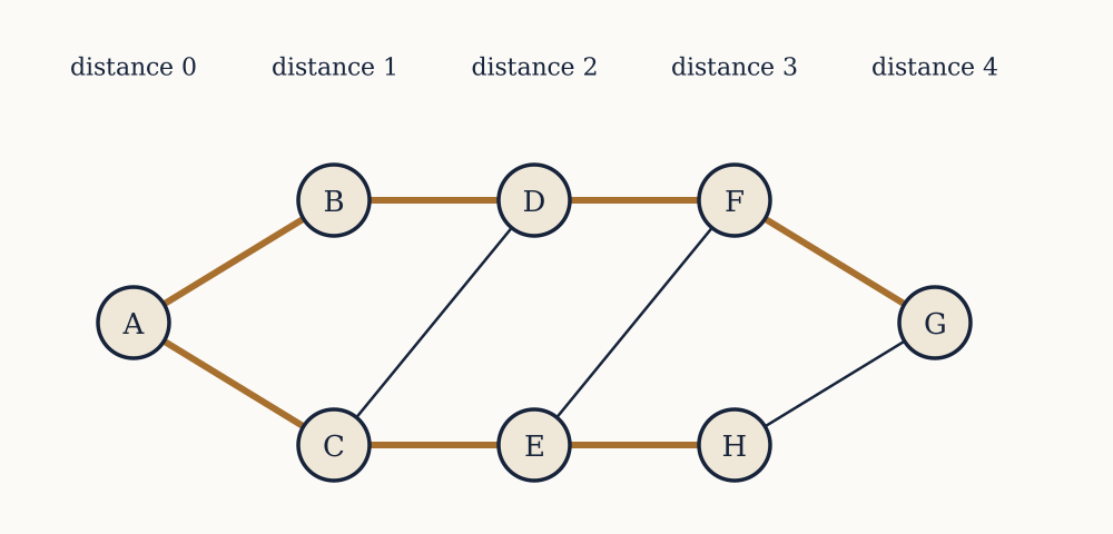
Now you. Run it from H instead.
Answer
H is 0. Its neighbours G and E are 1. From G comes F at 2, from E come C at 2 and F already found. From F comes D at 3, from C come D already found and A at 3. From D and A comes B at 4. Distances: H 0, G 1, E 1, F 2, C 2, D 3, A 3, B 4. Any one pair agrees in both directions, since A to H and H to A are both 3, but the table as a whole changes with the source: B was 1 from A and is 4 from H. What BFS computes is distance from one source, not a symmetric table.
Depth-first search
Depth-first search takes the newest pending vertex instead, which makes it a stack rather than a queue and, more naturally, a recursion: visit a vertex, then recursively visit each unvisited neighbour in turn. It plunges as deep as it can, backtracks when stuck, and plunges again.
The cost is the same , and it visits the same set of vertices, so as a reachability test the two are interchangeable. What differs is the structure they expose. BFS produces layers and shortest distances. DFS produces a nesting: each vertex has a discovery time and a finish time, and because the recursion is a stack, the intervals for any two vertices are either disjoint or one contains the other. That nesting is what makes DFS the tool for questions about structure rather than distance.
Colour each vertex white when unvisited, grey while its recursive call is on the stack, and black when finished. Then an edge from the current vertex to a grey vertex points back into the chain of calls that led here, which means a cycle. That is the whole of cycle detection: a directed graph has a cycle if and only if a depth-first search finds an edge to a grey vertex, and one traversal answers it in .
Topological order
A DAG describes things that must happen in some order, and the useful output is that order: a listing of the vertices in which every edge points forwards. It is called a topological order, and it exists exactly when the graph is acyclic, since a cycle would require a vertex to precede itself.
Two algorithms produce it. Kahn's, from 1962, is the more intuitive: compute every in-degree, put all the zero in-degree vertices in a ready set, and repeatedly remove one, output it, and decrement the in-degrees of its targets, adding any that reach zero. If the output is shorter than when the ready set empties, the remaining vertices form a cycle, so this detects cycles as a side effect. The DFS route is shorter to state: run a depth-first search and output vertices in reverse order of finishing time. It works because a vertex finishes only after everything reachable from it has finished.
Neither order is unique. Any vertex with no unmet prerequisite may go next, so a graph generally has many valid topological orders, and an algorithm may return any of them.
Example. A build has these dependencies: A must precede B and C, B must precede D, C must precede D and F, D must precede E, and F must precede E. Give a topological order by Kahn's algorithm, breaking ties alphabetically.
In-degrees are A 0, B 1, C 1, D 2, E 2, F 1. Only A is ready, so output A, which frees B and C. Output B, which decrements D to 1, not yet ready. Output C, which decrements D to 0 and frees F. Output D, which decrements E to 1. Output F, which decrements E to 0. Output E. The order is A, B, C, D, F, E, and every one of the six edges points forwards in it.
Now you. Add the requirement that E must precede C. Is there still a topological order?
Answer
No. C precedes D, D precedes E, and now E precedes C, so C must come before itself. Kahn's algorithm shows it mechanically: A is output and frees B, then B is output, and now nothing has in-degree zero, since C is waiting on E, D on C, E on D and F on C. The algorithm halts having output 2 of the 6 vertices, and that shortfall is the cycle report. A depth-first search would find it as an edge from E to the grey vertex C.
What this gives, and what it does not
Two traversals, both , answer a surprising number of questions. BFS gives reachability, connected components, the fewest-edge path between two vertices, and by running from both ends at once, the standard degrees-of-separation calculation. DFS gives cycle detection, topological order, and with a little more bookkeeping the strongly connected components, through Tarjan's 1972 algorithm or Kosaraju's, both still linear.
The limitation is in the word "fewest". BFS counts edges, and treats every edge as equally expensive. A road map is not like that: a route with three motorway segments beats one with two urban side streets, and the shortest path by distance may have many more edges than the shortest by count. The moment edges carry weights, BFS's ring-by-ring sweep is answering the wrong question, because the queue orders vertices by hop count and the cheapest route to a vertex may arrive later than the shortest one.
Fixing that means taking the pending vertex with the smallest accumulated cost rather than the one that has waited longest, which is to replace the queue with the priority queue built in the previous lesson. The next lesson does exactly that, proves that the resulting algorithm is correct only when weights are non-negative, gives the slower algorithm that survives negative ones, and then solves the related problem of connecting every vertex as cheaply as possible.