Shortest paths and spanning trees

Breadth-first search finds the route with the fewest edges, and on any graph whose edges carry a cost that is the wrong answer.

Three motorway segments beat two urban side streets, a flight with one connection may cost more than one with two, and a network path through four fast links beats one through two congested ones. The moment edges carry weights, "fewest" and "cheapest" come apart, and the sweep that made BFS correct, taking pending vertices in the order they were discovered, is exactly what stops working. This lesson repairs it, is precise about the condition under which the repair is valid, and then solves the closely related problem of wiring every vertex together as cheaply as possible.

Relaxation

Give every vertex an estimate $d [v]$ of its distance from the source, initially $0$ at the source and $\infty$ everywhere else. Every shortest-path algorithm in this lesson consists of repeating one operation until no estimate improves.

Relaxing the edge $(u, v)$ of weight $w$ means: if $d [u] + w < d [v]$ , then set $d [v] = d [u] + w$ and record $u$ as $v$ 's predecessor. In words, if going to $u$ and then taking this edge is cheaper than the best route to $v$ known so far, take it.

Two facts hold throughout. Every estimate is either infinite or the length of some real path, so no estimate is ever too small. And if $d [u]$ is already correct and the edge $(u, v)$ lies on a shortest path to $v$ , relaxing it makes $d [v]$ correct. The algorithms differ only in the order they relax edges: relax them in a bad order and the work repeats, in a good order and each edge is relaxed once.

The reason a good order exists is that shortest paths have optimal substructure: any subpath of a shortest path is itself a shortest path between its endpoints, since a cheaper subpath could be substituted to improve the whole. This licenses building long paths from short ones, and it is the same property the last two lessons of the course turn into a general technique.

Dijkstra's algorithm

Edsger Dijkstra designed this in 1956, by his own account in about twenty minutes in a cafe in Amsterdam, and published it in 1959.

The idea is to settle vertices in increasing order of true distance. Keep a set of settled vertices whose distances are final and a priority queue of the rest, keyed by their current estimate. Repeatedly extract the vertex with the smallest estimate, declare it settled, and relax all its outgoing edges.

The claim that makes this work is that when a vertex $u$ is extracted, $d [u]$ is already its true distance. Suppose not: then a genuinely shorter path to $u$ exists, and that path must leave the settled set somewhere, at some unsettled vertex $x$ . But $x$ has already been given an estimate by the relaxation that reached it, that estimate is at most the cost of the path's prefix up to $x$ , and that prefix is no longer than the whole path, which was assumed shorter than $d [u]$ . So $d [x] < d [u]$ and $x$ would have been extracted before $u$ . Contradiction.

Read that argument closely and the assumption is visible: the prefix is no longer than the whole path. That is true only if the remaining edges do not reduce the total, which is to say only if every weight is non-negative. Dijkstra's algorithm is correct under that condition and not otherwise.

The cost is one extraction per vertex and one possible decrease-key per edge. With the binary heap from the previous lesson that is $O ((V + E) \log V)$ , and on a sparse graph such as a road network, where $E \approx 3 V$ , that is close to $V \log V$ . With an array instead of a heap, extraction is $Θ (V)$ and the total is $Θ (V^{2})$ , which is actually faster on dense graphs.

Example. In an undirected graph with edges AB 4, AC 2, BC 1, BD 5, CD 8, CE 10, DE 2, DF 6 and EF 3, run Dijkstra from A.

A is settled at 0, relaxing B to 4 and C to 2. The smallest estimate is C at 2, which is settled; relaxing its edges improves B to $2 + 1 = 3$ , sets D to $2 + 8 = 10$ and E to $2 + 10 = 12$ . Next is B at 3, whose edge to D improves it to $3 + 5 = 8$ . Next is D at 8, which improves E to $8 + 2 = 10$ and sets F to $8 + 6 = 14$ . Next is E at 10, which improves F to $10 + 3 = 13$ . Finally F is settled at 13. The distances are A 0, C 2, B 3, D 8, E 10, F 13, and note that B was improved after its first estimate but before it was settled, which is the normal course of events.

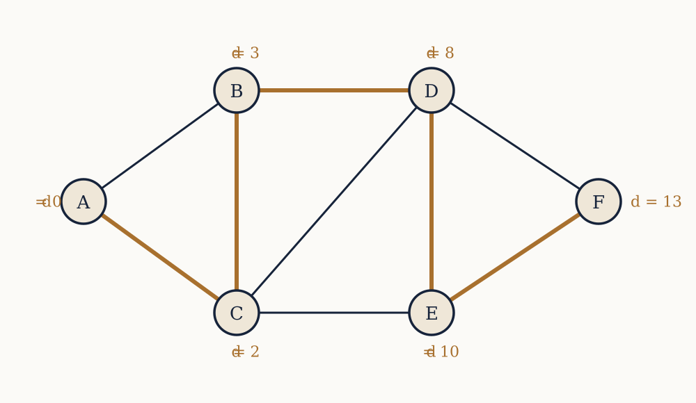
Now you. Run it from F on the same graph.

Answer

F settles at 0, giving E 3 and D 6. E settles at 3, improving D to $3 + 2 = 5$ and setting C to $3 + 10 = 13$ . D settles at 5, setting B to $5 + 5 = 10$ and leaving C at 13 since $5 + 8$ is also 13. B settles at 10, improving C to $10 + 1 = 11$ and setting A to $10 + 4 = 14$ . C settles at 11, improving A to $11 + 2 = 13$ . A settles at 13, agreeing with the previous run, as it must on an undirected graph.

When a weight is negative

Negative weights are not exotic. A currency exchange with a favourable rate, a chemical reaction that releases energy, a financial transaction with a rebate, a game move that gains points: all are edges with negative cost.

Example. A directed graph has A to B of weight 2, A to C of weight 5, and C to B of weight $- 4$ . What does Dijkstra return for B, and what is the truth?

Dijkstra settles A at 0, giving B an estimate of 2 and C an estimate of 5. The smallest is B at 2, so B is settled at 2 and never reconsidered. But the real cheapest route is A to C to B, costing $5 - 4 = 1$ . Dijkstra returns 2, and the answer is 1.

Now you. Does adding a large constant to every edge, to make them all non-negative, repair this?

Answer

No. Add 4 to each: A to B becomes 6, A to C becomes 9, C to B becomes 0. Now A to B costs 6 and A to C to B costs 9, so the two-edge route lost, when in the original graph it won. Adding a constant per edge penalises paths in proportion to their number of edges, which changes which path is shortest. Only a per-vertex reweighting preserves the ordering, which is exactly what Johnson's algorithm does, using the next algorithm to compute it.

Bellman-Ford, from Richard Bellman in 1958 and Lester Ford in 1956, gives up the ordering entirely and pays for it. Relax every edge in the graph, and repeat that $V - 1$ times. Since a shortest path has at most $V - 1$ edges, and each full pass over the edges correctly extends every shortest path by at least one more edge, $V - 1$ passes suffice. The cost is $Θ (V E)$ , which for a graph with a million vertices and three million edges is $3 \times 10^{12}$ operations against Dijkstra's $8 \times 10^{7}$ : about 40,000 times more.

Bellman-Ford also detects something Dijkstra cannot even define. If a $V$ -th pass still improves an estimate, the graph contains a negative cycle reachable from the source, and there is no shortest path at all, because going round the cycle again is always cheaper. That check is one extra pass and is the reason the algorithm is used to detect arbitrage in currency data.

Connecting everything, cheaply

A different problem on the same weighted graphs: choose a subset of edges connecting every vertex, with the least total weight. Wire a set of buildings, lay a pipe network, cluster a set of points.

The answer must be a tree. It has to be connected by requirement, and it cannot contain a cycle, since deleting any edge of a cycle leaves everything still connected and reduces the total. A connected acyclic subgraph touching every vertex is a spanning tree, and the cheapest one is a minimum spanning tree, with exactly $V - 1$ edges.

One fact settles both algorithms. Take any way of splitting the vertices into two non-empty parts, called a cut. The cheapest edge crossing that cut belongs to some minimum spanning tree. The proof is an exchange: take any minimum spanning tree not containing that edge $e$ , add $e$ , which creates exactly one cycle, and that cycle must cross the cut a second time at some edge $f$ . Remove $f$ . The result is still a spanning tree, and since $e$ was the cheapest crossing edge, its weight is no greater than $f$ 's, so the new tree is no more expensive. This is the cut property, and both algorithms are just different choices of which cut to apply it to.

Prim's algorithm, from Vojtěch Jarník in 1930 and rediscovered by Robert Prim in 1957, grows one tree. Start from any vertex, and repeatedly add the cheapest edge from the tree to a vertex outside it, using the cut between tree and non-tree. That is Dijkstra with a different key: the priority queue holds the cost of the cheapest single edge reaching a vertex rather than the cost of the whole path to it. The cost is likewise $O (E \log V)$ .

Kruskal's algorithm, from Joseph Kruskal in 1956, grows a forest. Sort all edges by weight, and take each in turn, adding it if its endpoints are in different components and discarding it otherwise. Each accepted edge is the cheapest crossing the cut between its own component and everything else, so the cut property applies. The sort costs $Θ (E \log E)$ and dominates.

Example. Run Kruskal on the graph above, with edges AB 4, AC 2, BC 1, BD 5, CD 8, CE 10, DE 2, DF 6 and EF 3.

Sorted: BC 1, AC 2, DE 2, EF 3, AB 4, BD 5, DF 6, CD 8, CE 10. Take BC, joining B and C. Take AC, joining A to them. Take DE. Take EF, giving a second component D, E, F. Reject AB, since A and B are already together. Take BD, which joins the two components into one containing all six vertices. That is five edges for six vertices, so the tree is complete and the remaining edges are never examined. Total weight $1 + 2 + 2 + 3 + 5 = 13$ .

Now you. Run it on the graph with edges PQ 7, PR 5, QR 8, QS 9, RS 15, RT 6, ST 8, SU 5 and TU 11.

Answer

Sorted: PR 5, SU 5, RT 6, PQ 7, QR 8, ST 8, QS 9, TU 11, RS 15. Take PR, take SU, take RT, take PQ. Reject QR, since Q and R are both in the component P, Q, R, T. Take ST, which merges S, U with that component, giving all six vertices in five edges. Total weight $5 + 5 + 6 + 7 + 8 = 31$ . Prim's algorithm from P would take the same five edges in the order PR, RT, PQ, ST, SU, which is a different order and the same tree.

Union-find

Kruskal's rejection test asks, for each edge, whether two vertices are already in the same component, and merges two components when they are not. Done naively, by relabelling every vertex of one component, a single merge costs $Θ (V)$ and the algorithm becomes quadratic.

The structure that does it properly is union-find, also called disjoint-set. Each component is a tree of parent pointers whose root names the set. find(x) walks to the root; union(x, y) links one root under the other. Two refinements make it fast. Union by rank always links the shorter tree under the taller, keeping heights logarithmic. Path compression makes every node visited by a find point directly at the root afterwards, so the walk pays for itself.

With both, a sequence of $m$ operations on $n$ elements costs $O (m α (n))$ , where $α$ is the inverse Ackermann function, proved by Robert Tarjan in 1975. That function grows so slowly that $α (n) \leq 4$ for every $n$ up to $2^{65536}$ . The cost is not constant, and Tarjan also proved that no structure can make it constant, but it is below any threshold that will ever be measured, so in Kruskal it is negligible against the sort.

What is settled and what is not

Shortest paths from one source cost $O ((V + E) \log V)$ with non-negative weights and $Θ (V E)$ without them. All pairs can be had by running Dijkstra from every vertex, or in $Θ (V^{3})$ by Floyd and Warshall's 1962 triple loop over an adjacency matrix, which is better on dense graphs. Minimum spanning trees cost $O (E \log V)$ either way.

Something the three algorithms have in common is worth naming. Dijkstra takes the vertex with the smallest estimate. Prim takes the cheapest edge leaving the tree. Kruskal takes the cheapest edge overall. In every case the algorithm takes the locally best option available and never goes back to reconsider it, and in every case the result is provably optimal.

That is remarkable, and it is not general. Taking the locally best option is a strategy that usually fails, and each of these algorithms needed its own argument, the cut property or the settling argument, to show that it does not. The next lesson names the strategy, states what has to be proved for it to be trusted, and shows a problem, one sentence away from a problem it solves perfectly, where it fails.