Probability

Uncertainty is not the same thing as ignorance, because some uncertain things are more uncertain than others, and that comparison is what a number is for. This lesson asks what such a number could possibly mean, gets two incompatible answers, and finds that both answers obey the same rules. Nothing here needs more than arithmetic and the algebra of the foundations course.

The rule that started it

The oldest working definition of probability is a ratio of counts. List every case the situation can produce, decide which of them count as the event you care about, and divide:

Gerolamo Cardano wrote this down in his Liber de Ludo Aleae around 1564, sitting on the manuscript until it was printed in 1663, and Pierre-Simon Laplace made it the formal definition in 1812 with one crucial rider: the cases must be equally possible. With that rider the rule works. A fair die has six cases, one of which is a six, so $P(\text{six})=1/6\approx 0.1667$. Two dice have $6\times 6=36$ cases, of which six sum to seven, so $P(\text{sum}=7)=6/36\approx 0.1667$ as well, while only five sum to eight, giving $5/36\approx 0.1389$.

That last pair of numbers is already worth something, because it explains an observation gamblers had made for centuries without being able to justify: seven comes up more often than eight, even though both can be made in several ways. The counting has to be done over the $36$ ordered pairs, not over the $21$ unordered totals, and the whole history of early probability is people getting that distinction wrong.

Two games that differ by a hair

In 1654 Antoine Gombaud, who styled himself the Chevalier de Méré, put a complaint to Blaise Pascal. He made money betting that at least one six would appear in four rolls of a single die, and lost money betting that at least one double six would appear in twenty-four rolls of two dice. His reasoning said the two should be identical: one chance in six, four rolls, and one chance in thirty-six, twenty-four rolls, both giving four sixths of a certainty. His purse said otherwise.

The counting rule settles it, provided you count the failures rather than the successes. Four rolls of one die produce $6^4=1296$ equally likely sequences, and $5^4=625$ of them contain no six, so

Twenty-four rolls of a pair produce ${36}^{24}$ sequences, of which ${35}^{24}$ avoid the double six, so

One game is a shade better than even and the other a shade worse. The gap is $0.0263$, about one bet in thirty-eight, which is invisible over an evening and ruinous over a career. De Méré had played enough to feel a difference of two and a half percentage points. The correspondence between Pascal and Fermat that followed this question is where the subject begins.

Example. What is the probability of getting at least one six in five rolls of a fair die?

Count the failures. Each roll avoids a six in five of its six cases, and the rolls are laid out as a sequence, so $5^5=3125$ of the $6^5=7776$ sequences contain no six at all. The complement gives $1-3125/7776=4651/7776\approx 0.5981$.

Now you. What is the probability of getting at least one six in three rolls of a fair die?

Where counting cases runs out

The classical rule has two faults, and neither is repairable from inside it.

The first is circularity. "Equally possible" means equally probable, so the definition of probability contains the word it is defining. For a die this is harmless, because the symmetry of a cube gives an independent reason to believe the six cases are interchangeable: relabel the faces and nothing physical changes. Away from manufactured symmetric objects the escape closes. A drawing pin tossed on a table lands point up or point down, which is two cases, and nobody believes the answer is $1/2$. Nothing about the pin says the two cases are interchangeable, and the only way to find out is to throw it.

The second fault is that the rule is silent whenever the cases cannot be made symmetric at all. What is the probability that a particular patient survives five years, that a bridge design fails, that it rains tomorrow? There is no bag of equally possible cases to count. These are the questions people actually have, and the classical definition does not so much answer them badly as refuse to accept them.

So the counting rule is not a definition. It is a correct calculation for one special structure, a finite space of interchangeable outcomes, and the general notion has to come from somewhere else.

What the record actually shows

The obvious somewhere else is measurement. If the probability of heads is the fraction of heads in the long run, then the way to find it is to toss the coin many times. People have done exactly this. Georges-Louis Leclerc, Comte de Buffon, recorded $2048$ heads in $4040$ tosses. Karl Pearson recorded $12012$ in $24000$. The most careful record is John Kerrich's, made while interned in Denmark during the Second World War and published in 1946, and it is worth seeing in full because it shows two things at once.

Read the third column and the coin looks worse and worse: Kerrich ends $67$ heads clear of half, having been only $6$ clear at a hundred tosses. Read the fourth and it looks better and better, closing on $0.5$ from $0.44$. Both columns are correct, and they are not in conflict. The absolute surplus of heads grows without limit while the surplus divided by the number of tosses shrinks towards nothing. Whichever of these you call "the coin settling down" determines what you think probability is, and the later lesson on the laws of large numbers gives the exact rate at which each happens.

The fatal difficulty with defining probability as the long-run fraction is in the phrase "long run". No finite record ever hands you a number: Kerrich's fraction was $0.5067$, not $0.5$, and another ten thousand tosses would have given a third value. To say the fraction tends to a limit is to make a claim no experiment can confirm, and worse, it is a claim that is not even guaranteed by the theory, since a fair coin can in principle give heads forever. Frequency tells you how to estimate a probability. It does not tell you what one is.

Example. Kerrich was $6$ heads below half at a hundred tosses and $67$ above at ten thousand. In which record was the coin behaving more like a fair one?

Compare fractions, not counts. At a hundred tosses the fraction was $44/100=0.44$, which misses $0.5$ by $0.06$. At ten thousand it was $5067/10000=0.5067$, missing by $0.0067$, roughly nine times closer. The larger discrepancy in raw heads belongs to the far larger experiment, and it is the fraction that carries the information about the coin.

Now you. At one thousand tosses Kerrich had $502$ heads. Give the fraction and its distance from $0.5$, and say how it compares with the ten thousand toss figure.

Probability as a price

The third reading abandons repetition altogether. On this view a probability is a degree of belief, and it is measured the way beliefs have always been measured in practice, by what someone will bet. Frank Ramsey in 1926 and Bruno de Finetti in 1931 made this precise. If you regard a payout of one unit on event $A$ as worth exactly $p$ units to buy or to sell, then $p$ is your probability for $A$.

This sounds like an invitation to say anything, and it is not, because inconsistent prices can be robbed. Bookmakers quote odds "against": at $3$ to $1$ against, a winning stake of $1$ returns $4$, which corresponds to a probability of $1/(3+1)=0.25$. Suppose a race with three horses is priced at $2$ to $1$, $3$ to $1$ and $4$ to $1$ against. The implied probabilities are $1/3$, $1/4$ and $1/5$, and they sum to $0.7833$. Back all three, staking exactly those fractions of a unit. Whichever horse wins, the return is exactly $1$, because $3\times \frac{13}{=}4\times \frac{14}{=}5\times \frac{15}{=}1$. Total outlay $0.7833$, guaranteed return $1$, guaranteed profit $0.2167$ per unit staked out, a return of $27.7$ percent on money with no risk whatsoever.

A set of prices that permits this is called a Dutch book, and the theorem that Ramsey and de Finetti proved is that you are safe from one if and only if your prices lie between $0$ and $1$ and add to exactly $1$ across a set of alternatives exactly one of which must happen. Coherence, not frequency, forces the arithmetic. Real bookmakers make the sum exceed $1$ on purpose, and the excess is their margin.

Example. A market prices three outcomes at evens ($1$ to $1$), $5$ to $1$ and $9$ to $1$ against. Is it coherent, and if not, what is the risk-free return?

The implied probabilities are $1/2$, $1/6$ and $1/10$, summing to $0.7667$, which is less than $1$, so the market is incoherent in the punter's favour. Staking $0.5$, $0.1667$ and $0.1$ returns exactly $1$ whichever outcome occurs, for an outlay of $0.7667$: a profit of $0.2333$ per unit returned, which is $30.4$ percent on the money staked.

Now you. A two-outcome market is priced at $2$ to $1$ against on each side. What do the implied probabilities sum to, and who can be robbed?

What both readings share

The frequentist reads a probability as a fact about a repeatable setup, and refuses to assign one to a unique event. The Bayesian reads it as a coherent price, and assigns one to anything. They disagree about what the number means, and about which questions are legitimate. They do not disagree about the arithmetic, and this is the fact the rest of the subject is built on.

Both give every probability a value in $[0,1]$, because a fraction of a total cannot be negative or exceed the whole, and a price outside that range is a Dutch book in one line. Both make the probabilities of a set of mutually exclusive alternatives, one of which must occur, sum to exactly $1$: the counting rule because the favourable cases partition the total, the betting rule because coherence demands it. Both make the probability of "$A$ or $B$" equal to the sum of the separate probabilities when $A$ and $B$ cannot both happen, since disjoint sets of cases add and so do the stakes that cover them.

That is three rules, and they were reached three times over from unrelated starting points. Andrey Kolmogorov's move in 1933 was to stop asking what probability is and take those three statements as axioms, with everything else to be proved from them. It is the same move that made group theory out of symmetry and metric spaces out of distance, and it is why probability became a branch of mathematics rather than a collection of gambling results.

What is still missing

Taking the rules as axioms leaves an obvious gap. Rules have to be rules about something, and every statement above quietly assumed a background list: the six faces, the $1296$ sequences, the three horses. "The probability of $A$ or $B$" only means anything once $A$ and $B$ are the kind of object that can be combined with "or" at all.

So the first construction the subject needs is not a formula but a set: the collection of everything that could happen, with events living inside it as subsets, and "or", "and" and "not" becoming union, intersection and complement. That is the next lesson, and it turns the three rules above into three axioms with enough structure that real theorems follow from them.

Three rules survived the previous lesson: probabilities lie between zero and one, the alternatives sum to one, and disjoint alternatives add. Rules need something to be rules about, and this lesson builds it. The construction is set theory of the plainest kind, and by the end of it a handful of genuinely useful formulas will have been proved rather than asserted.

The list of everything that can happen

Start with the experiment, meaning any procedure with an uncertain result. Its sample space $\Omega$ is the set of all its possible outcomes, chosen so that exactly one of them occurs on each run: no two can happen together, and none can be left out.

For one roll of a die, $\Omega =\{1,2,3,4,5,6\}$. For two dice distinguished by colour, $\Omega$ is the set of ordered pairs $(i,j)$, so it has $36$ elements. That choice is not forced, and the alternative is instructive: you could take $\Omega$ to be the $11$ possible totals, from $2$ to $12$, and the definition would still be satisfied, since exactly one total occurs. What you lose is symmetry. The $36$ pairs are interchangeable and the $11$ totals are not, so only the first choice lets you count. Choosing a sample space fine enough to be symmetric is the single most useful habit in the subject.

Sample spaces need not be finite. Toss a coin until the first head appears and record how many tosses it took: $\Omega =\{1,2,3,\dots \}$, countably infinite, with no upper bound on how long you might wait. Measure the lifetime of a light bulb in hours and $\Omega$ is the set of non-negative real numbers, uncountable. All three kinds appear in this course.

An event is a subset of $\Omega$: any collection of outcomes you might want to speak about as a unit. "The die shows an even number" is the subset $\{2,4,6\}$. "The two dice total seven" is a subset of six pairs. An event occurs when the outcome that happened is one of its members. Individual outcomes give the one-element events, $\Omega$ itself is the certain event, and the empty set $\varnothing$ is the impossible one.

Or, and, not

Putting events in a set makes ordinary logical words into set operations, and this is the whole reason for the construction.

"$A$ or $B$", meaning at least one of them, is the union $A\cup B$. "$A$ and $B$", meaning both, is the intersection $A\cap B$. "Not $A$" is the complement $A^c=\Omega \setminus A$. Two events with $A\cap B=\varnothing$ cannot both occur and are called disjoint or mutually exclusive. A family of events that are pairwise disjoint and whose union is all of $\Omega$ is a partition: exactly one of them happens.

Set algebra now supplies identities for free, including the two of De Morgan:

Read in words, the first says that "neither happened" is the same statement as "not the first and not the second", and the second says that "they did not both happen" is the same as "at least one failed to". These are not probability facts, they are facts about sets, and they will convert several awkward calculations into easy ones. The trick that solved de Méré's dice problem in the previous lesson was exactly the first identity: "at least one six" is the complement of "no sixes", and the second is far easier to count.

Three axioms

Kolmogorov's 1933 axioms assign to each event $A$ a number $P(A)$ subject to three demands.

The third is countable additivity, and the word countable is doing real work: it holds for infinite sequences of disjoint events, not merely for finitely many. That extension is what allows the coin-until-heads space to be handled, where the probabilities $1/2,1/4,1/8,\dots$ must sum to $1$ over infinitely many outcomes, which they do by the geometric series.

One honest caveat. On an uncountable sample space, such as a dart landing anywhere on a metre rule, it is not possible to assign a sensible probability to every subset: there are subsets so pathological that any assignment contradicts the axioms. The repair is to declare in advance a family of subsets that count as events, closed under complement and countable union, and demand nothing about the rest. That family is called a $\sigma$-algebra, and for everything in this course it can be ignored, because every set anyone would write down is in it. It is mentioned here only so that the word is not a surprise elsewhere.

What follows at once

Everything below is proved from the three axioms and nothing else.

The complement rule comes first. $A$ and $A^c$ are disjoint and their union is $\Omega$, so $P(A)+P(A^c)=P(\Omega )=1$, giving

Take $A=\Omega$ and this gives $P(\varnothing )=0$: the impossible event has probability zero. The converse fails, and it will matter later. An event of probability zero need not be impossible, as the lesson on continuous variables shows.

Next, if $A\subseteq B$, split $B$ into the disjoint pieces $A$ and $B\setminus A$. Then $P(B)=P(A)+P(B\setminus A)$, and since the last term cannot be negative,

so probability is monotone. Combined with $P(\Omega )=1$ this bounds every probability above by one, which the axioms never stated directly. The rearrangement $P(B\setminus A)=P(B)-P(A)$ is the difference rule, valid when $A$ sits inside $B$ and not otherwise.

Example. In a group, $70$ percent own a bicycle and $40$ percent own a bicycle and a car. What can be said about the percentage owning a bicycle but no car?

"Bicycle and car" is a subset of "bicycle", so the difference rule applies exactly: $P(\text{bicycle},\text{no car})=0.70-0.40=0.30$. Note that nothing was assumed about how the two ownerships relate. The subset relation did all the work.

Now you. In the same group, $55$ percent own a car. What percentage own a car but no bicycle?

Adding events that overlap

The third axiom adds probabilities only for disjoint events, and most interesting pairs overlap. Fix it by splitting.

Write $A\cup B$ as the two disjoint pieces $A$ and $B\setminus (A\cap B)$. Additivity gives $P(A\cup B)=P(A)+P(B\setminus (A\cap B))$, and since $A\cap B\subseteq B$ the difference rule turns the second term into $P(B)-P(A\cap B)$. Hence

This is inclusion and exclusion. The subtraction is bookkeeping: adding the two probabilities counts the overlap twice, so it comes off once. For three events the same argument, applied twice, gives

The pattern continues, alternating in sign, with all singles added, all pairs subtracted, all triples added, and so on.

Dropping the subtractions leaves an inequality that holds always, since the terms removed are non-negative:

This is the union bound, or Boole's inequality. It is crude, it needs no information at all about how the events relate, and it is used constantly, because "at least one of these bad things happens" is bounded by the sum of the individual risks whether or not they are connected. When the sum exceeds one it says nothing, which is the honest signal that the events overlap too much for it to help.

Example. A whole number is drawn at random from $1$ to $1000$, each equally likely. What is the probability it is divisible by $2$, by $3$ or by $5$?

Count each set: $500$ multiples of $2$, $333$ of $3$, $200$ of $5$. Subtract the pairs, counted by the least common multiples: $166$ multiples of $6$, $100$ of $10$, $66$ of $15$. Add back the $33$ multiples of $30$. The union has

members, so the probability is $0.734$. The union bound would have offered only $\le (500+333+200)/1000=1.033$, which is no information at all.

Now you. Two fair dice are rolled. Let $A$ be "at least one die shows a five", which contains $11$ of the $36$ pairs, and $B$ be "the total is eight", which contains $5$. Their intersection contains $2$. Find $P(A\cup B)$.

When the outcomes are equally likely

Suppose $\Omega$ is finite with $N$ outcomes and all of them carry the same probability $p$. Additivity over the $N$ one-element events gives $Np=P(\Omega )=1$, so $p=1/N$, and for any event $A$ containing $|A|$ outcomes,

The classical rule of the previous lesson is recovered, no longer as a definition but as a theorem about one particular assignment among many. The axioms are silent about whether the outcomes deserve equal probability; that is a modelling decision made outside the mathematics, justified by symmetry when there is symmetry and by measurement when there is not.

Nothing forces uniformity. A loaded die might carry $P(6)=0.25$ with the other five faces sharing the remaining $0.75$ equally, at $0.15$ each, and every rule above still applies unchanged. The infinite space is the sharper case: for the coin tossed until the first head, $P(n)=2^{-n}$, which sums to $1$ but assigns different probabilities to different outcomes, and no uniform assignment on $\{1,2,3,\dots \}$ is even possible, since equal positive values summing to one over infinitely many outcomes cannot exist.

Example. A die is loaded so that $P(6)=0.25$ and the other five faces are equally likely. What is the probability of an even number?

The other five faces share $1-0.25=0.75$, so each has $0.15$. The even faces are $2$, $4$ and $6$, disjoint one-element events, so $P(\text{even})=0.15+0.15+0.25=0.55$. On a fair die it would be $0.5$, and the loading has shifted it.

Now you. For the same loaded die, find the probability that the result is at least $4$.

What the axioms do not give you

Three axioms and some set algebra have produced the complement rule, monotonicity, the difference rule, inclusion and exclusion in any number of events, and the union bound. That is a working toolkit, and it is worth being clear about what it is not.

The axioms never say what number to attach to any particular event. They constrain assignments to be consistent with one another; they cannot manufacture one out of nothing. Every calculation in this lesson began from probabilities that were either handed over or justified by a symmetry argument outside the theory, and this is not a defect to be repaired later. It is the permanent division of labour: modelling supplies the inputs, the axioms police the consequences.

The other gap is practical. Once symmetry does apply, $P(A)=|A|/N$ reduces every question to two counts, and the sets that arise are rarely small enough to list. How many five-card hands contain two pairs? How many ways can twenty-three birthdays fall so that no two coincide? Answering questions like these is a discipline of its own, and it is the subject of the next lesson.

When outcomes are equally likely, a probability is a ratio of two counts, and the counts are rarely small enough to list. This lesson builds the three tools that do the counting, checks them against a deck of cards, and then uses them on a question whose true answer almost nobody guesses within a factor of two.

Choices in sequence

Everything here rests on one observation. If a first choice can be made in $a$ ways and, for each of those, a second in $b$ ways, then the pair can be made in $ab$ ways. Lay the possibilities out as a rectangular grid with $a$ rows and $b$ columns and the claim is just the area of a rectangle. Extend to any number of stages and it becomes the product rule: multiply the number of options at each stage, provided the number of options at each stage does not depend on which options were taken earlier.

That proviso is the whole art. Two dice give $6\times 6=36$ sequences because the second die does not care what the first did. A four-character password from the $26$ lowercase letters gives ${26}^4=456976$, again because letters may repeat. But drawing two cards from a deck gives $52\times 51=2652$ ordered pairs, not ${52}^2$, because the second draw has one fewer option: the count at each stage changed, though crucially it changed by the same amount regardless of which card went first, and that is enough for the rule to apply.

Sampling with replacement leaves the pool intact and gives $n^k$ sequences of length $k$. Sampling without replacement shrinks it and gives $n(n-1)(n-2)\cdots (n-k+1)$, a product of $k$ falling terms. When $k=n$ the second product uses up the whole pool and is written $n!$, read "$n$ factorial", with $0!=1$ by the convention that there is exactly one way to arrange nothing.

Ordered selections

The falling product has a name. The number of permutations of $k$ items chosen from $n$ distinct items, where order matters and nothing is reused, is

The second form is the first with the unused tail $(n-k)!$ divided away, which is often the easier thing to compute. The five-card deal from a shuffled deck, if you insist on tracking the order they arrived in, gives $P(52,5)=52\times 51\times 50\times 49\times 48=311875200$ possibilities.

Repeated items collapse the count. The letters of MISSISSIPPI can be arranged in $11!$ ways if the letters are all treated as distinct, but the four S's are not distinguishable, so every genuine arrangement has been counted $4!$ times over on their account, and likewise $4!$ for the I's and $2!$ for the P's. Divide those out:

That division, cancelling the orderings you did not want to distinguish, is the single most useful move in combinatorics, and the next section is nothing but the same move applied once.

Unordered selections

A poker hand is a set of five cards, and the order it was dealt in is nobody's business. Each such set of five was counted $5!$ times among the $311875200$ ordered deals, once for each arrangement of the same five cards. So the number of distinct hands is that figure divided by $5!=120$, giving $2598960$.

In general the number of ways to choose $k$ items from $n$ when order is irrelevant is written $C(n,k)$, read "$n$ choose $k$", and

Two properties are worth carrying. First, $C(n,k)=C(n,n-k)$, because choosing which $k$ to take is the same act as choosing which $n-k$ to leave. Second, $C(n,k)=C(n-1,k-1)+C(n-1,k)$: fix any one item, and every selection either includes it, which leaves $k-1$ to pick from the other $n-1$, or excludes it, which leaves $k$ to pick from the other $n-1$. That identity generates Pascal's triangle row by row, and it will return in the lesson on the binomial distribution.

Example. A lottery draws $6$ numbered balls from $49$, order irrelevant. What is the probability that one particular ticket matches all six?

The number of possible draws is $C(49,6)=49!/(6!43!)=13983816$, and exactly one is the ticket, so the probability is $1/13983816\approx 7.15\times {10}^{-8}$. Buying one ticket a week, the expected wait for a win is about $269000$ years.

Now you. How many ways are there to choose a committee of $3$ people from a group of $10$, and what is the probability that a randomly chosen committee contains one particular person?

Poker as a test bench

A ranked list of poker hands is a good check on the machinery, because the ranking was fixed by players long before anyone computed it, and the counts must come out in the same order.

Take two pair. Choose the two ranks that will be paired: $C(13,2)=78$ ways. Choose two suits for each of them: $C(4,2)=6$ ways each, so $36$. The fifth card must avoid both chosen ranks, leaving $52-8=44$ cards. That gives $78\times 36\times 44=123552$ hands, and

Note the order of the two ranks was never used, which is why $C(13,2)$ and not $13\times 12$ appears. Choosing "kings and threes" is the same hand as choosing "threes and kings", and counting it twice would double the answer.

Now a flush. Choose a suit, $4$ ways, then any five of its $13$ cards, $C(13,5)=1287$ ways, giving $5148$. Of those, $40$ are also straights and are ranked higher, so a plain flush has $5108$ hands and probability $5108/2598960\approx 0.0020$. Two pair is about $24$ times commoner than a flush, and duly ranks below it. The same method gives $3744$ full houses ($\approx 0.0014$) and $624$ four-of-a-kinds ($\approx 0.00024$), and the ranking players arrived at by experience is exactly the ranking these counts produce.

Example. How many five-card hands are three of a kind, meaning exactly three cards of one rank and two other cards of two different ranks?

Pick the tripled rank in $13$ ways and its three suits in $C(4,3)=4$ ways. The other two cards must be of two distinct ranks, neither equal to the first: $C(12,2)=66$ choices of ranks, and $4\times 4=16$ choices of suit. That gives $13\times 4\times 66\times 16=54912$ hands, a probability of about $0.0211$.

Now you. How many five-card hands contain exactly one pair, meaning two cards of one rank and three others of three different ranks?

The birthday problem

Take $23$ people at random. What is the probability that two of them share a birthday? The usual guess is a few percent, on the grounds that $23$ is small next to $365$. The right answer is slightly over one half.

Count the complement, as always. Ignore leap years and assume all $365$ days equally likely, an assumption examined below. Sequences of $23$ birthdays number ${365}^{23}$, all equally likely. Those with no repeat are ordered selections without replacement, $365\times 364\times \cdots \times 343$, so

and the probability of at least one shared birthday is $1-0.4927=0.5073$.

The reason intuition fails is that people compare $23$ with $365$, when the right comparison is with the number of pairs. Twenty-three people form $C(23,2)=253$ pairs, and $253$ against $365$ no longer looks small. Each pair matches with probability $1/365$, so the union bound of the previous lesson caps the answer at $253/365\approx 0.693$, which is loose but already in the right neighbourhood, and it is loose in the right direction: the pairs overlap heavily, since any three people share three pairs among them.

The curve climbs fast. Ten people give $0.117$, thirty give $0.706$, fifty give $0.970$. The real-world assumption of uniform birthdays is not quite true, with seasonal peaks and a deficit around late December in many countries, but the effect only ever pushes the probability up, since any unevenness makes coincidences commoner. The $23$ figure is therefore a safe upper bound on the number of people needed.

Example. What is the probability that among $10$ people at least two share a birthday?

Multiply the falling ratios: $P(\text{no match})=\prod _{k=0}^9(365-k)/365\approx 0.8831$, so the answer is $1-0.8831=0.1169$, about one chance in nine. Small, but far larger than the $10/365\approx 0.027$ that a careless comparison suggests.

Now you. Four fair dice are rolled. What is the probability that at least two show the same number?

What counting assumes, and when it stops working

Every calculation above began by declaring a set of equally likely outcomes and then measuring a subset of it. That is a strong assumption, and it is doing more work than the algebra. If the deck is not well shuffled, or the birthdays are not uniform, or the lottery machine favours a ball, the counts are still right and the probabilities are wrong. Counting is a technique for evaluating a model, not evidence that the model is correct.

There is a second and sharper limit. The whole method treats the sample space as intact: all $2598960$ hands are live, all ${365}^{23}$ birthday sequences are live. The moment any information arrives, most of them are not. Told that the first two cards dealt are aces, the remaining possibilities are a much smaller set, and the probability of four of a kind is no longer $0.00024$. Told that one person in the room was born in March, the birthday calculation changes.

Recounting from scratch after every piece of news is unworkable, and it is also unnecessary, because the effect of information on a probability follows one rule that can be derived once. Deriving it, and finding that it makes independence into a definition rather than a feeling, is the next lesson.

Every probability computed so far assumed the whole sample space was still in play, and information destroys that assumption. This lesson derives the one rule that says what a probability becomes once something is known, and then uses it to define independence, to build trees, and to settle a game show argument that split a magazine's readership in 1990.

Renormalising onto what is left

Two fair dice are rolled and you are told the total is at least nine. What is the probability that at least one die shows a six?

The original sample space had $36$ equally likely pairs. The news has killed every pair whose total is eight or less, leaving $10$ pairs, and those $10$ are still equally likely relative to one another, because nothing distinguished them before and the news treated them alike. Of the survivors, $7$ contain a six. So the answer is $7/10=0.7$, against an unconditional $11/36\approx 0.306$.

Two things happened. The sample space shrank to the event that was reported, and the probabilities of the survivors were scaled up so they again sum to one. That scaling is a division by the probability of the reported event, and writing it in general gives the definition. For events $A$ and $B$ with $P(B)>0$,

read "the probability of $A$ given $B$". The numerator keeps only the part of $A$ that survives, and the denominator is the renormalisation. Check it on the dice: $P(A\cap B)=7/36$, $P(B)=10/36$, and the ratio is $7/10$.

This is a definition rather than a theorem, but it is not arbitrary. For any fixed $B$, the assignment $A\mapsto P(A|B)$ satisfies all three of Kolmogorov's axioms: it is non-negative, it gives $\Omega$ probability $P(B)/P(B)=1$, and it is additive because the numerator is. So a conditional probability is a probability, and every rule from the earlier lesson holds inside it, including $P(A^c|B)=1-P(A|B)$. What is not true, and is a standard error, is that anything holds when you condition on different things: $P(A|B)+P(A|B^c)$ is not $1$ and need not be anything in particular.

The chain rule

Multiply the definition out and it becomes a way to build probabilities rather than to update them:

and iterating, for three events,

This is how sequential experiments are actually computed. Draw two cards from a full deck: the first is an ace with probability $4/52$, and given that, the second is an ace with probability $3/51$, since one ace and one card are gone. So

Three aces adds a factor $2/50$ and gives $\approx 0.000181$. The counting lesson would reach the same answers through $C(4,2)/C(52,2)$, and the chain rule is usually quicker because each factor is a small local question.

The same pattern handles any sequential draw. An urn holding $5$ red and $3$ black balls gives up two reds in a row with probability $(5/8)(4/7)=20/56\approx 0.3571$, and two blacks with probability $(3/8)(2/7)=6/56\approx 0.1071$, each factor asking only what is left in the urn at that moment.

Independence, defined rather than felt

Sometimes the news changes nothing: $P(A|B)=P(A)$. Substituting into the chain rule turns this into a symmetric statement with no division in it, and that is the form to take as the definition. Events $A$ and $B$ are independent when

The symmetry is worth noticing. If $B$ tells you nothing about $A$ then $A$ tells you nothing about $B$, which is not obvious from the conditional form but is immediate from this one. The definition also handles the awkward case $P(B)=0$, where the conditional is undefined but the product form is fine.

Independent is not the same as disjoint, and confusing them is the commonest slip in the subject. Disjoint events are maximally dependent: if $A$ and $B$ cannot both happen, then learning $B$ occurred tells you $A$ certainly did not, so $P(A|B)=0$. Two disjoint events of positive probability are never independent.

Independence is also not settled by checking pairs. Roll two fair dice and take $A$ as "first die is even", $B$ as "second die is even", $C$ as "the total is even". Each has probability $1/2$, and each pair is independent: knowing the first die is even says nothing about the second, and knowing the second die is even leaves the total even exactly when the first is, still probability $1/2$. But the three together are not independent, because any two of them force the third, so $P(A\cap B\cap C)=P(A\cap B)=1/4$, not $(1/2{)}^3=1/8$. Full independence of a family means every subfamily multiplies, not merely every pair.

In practice independence is an assumption imported from the physics of the situation, not something read off the numbers. Successive coin tosses are independent because a coin has no memory. Successive days of rain are not. Assuming independence where it does not hold is how risk models fail, since it makes simultaneous disasters look astronomically unlikely when they are merely unlikely.

Example. A component fails during a mission with probability $0.02$, independently of the other components. A system contains four such components and works only if all four survive. What is the probability that the system works?

Independence lets the probabilities multiply: $P(\text{all survive})={0.98}^4\approx 0.9224$, so the system fails with probability about $0.0776$, nearly four times the single-component risk.

Now you. The same system is built with six such components instead of four. What is the probability that it works?

The law of total probability

Conditioning is most useful when the conditioning events form a partition: a set of alternatives $B_1,B_2,\dots ,B_n$, exactly one of which occurs. Any event $A$ is then chopped into the disjoint pieces $A\cap B_i$, and additivity plus the chain rule gives

the law of total probability. Read it as an instruction: split the world into cases, work out the answer within each case, and average the answers weighted by how likely each case is.

Take a factory with three machines. Machine one makes $50$ percent of the output with a defect rate of $1$ percent, machine two makes $30$ percent at $2$ percent, machine three makes $20$ percent at $3$ percent. An item is picked at random from the day's production. Then

so $1.7$ percent overall, which lies between the best and worst machine rates and is nearer the best, because the best machine makes the most. Note what the calculation does not answer: given that an item is defective, which machine most likely made it? Machine one contributes the largest single share of the defects, $0.005$ out of $0.017$, or $29.4$ percent, despite having the lowest defect rate, simply because it makes half of everything. That reversal is the subject of the next lesson.

Example. From the urn of $5$ red and $3$ black balls, two are drawn without replacement. What is the probability that the second is red?

Condition on the first. If the first was red (probability $5/8$), four of the remaining seven are red. If it was black (probability $3/8$), five of seven are. So

which is exactly $5/8$, the probability the first is red. This is not a coincidence: before you look at anything, the ball in position two is as likely to be red as the ball in position one, because the balls were never ordered by colour. Symmetry gives the answer in one line where conditioning takes three.

Now you. A box holds $4$ white and $6$ green counters. Two are drawn without replacement. Use the law of total probability to find the probability that the second is white, and check it against the symmetry argument.

The three doors

In September 1990 Marilyn vos Savant answered a reader's question in Parade magazine and received thousands of letters telling her she was wrong, many from people with doctorates. The setup: three doors, a car behind one and goats behind the other two. You pick a door. The host, who knows where the car is, opens one of the other two to reveal a goat, and always can. He offers you the switch. Should you take it?

The answer is yes, and switching wins with probability $2/3$. The clean way to see it is to condition on your first pick, which is the only random thing you control. With probability $1/3$ your first pick was the car, in which case switching loses. With probability $2/3$ it was a goat, in which case the host is forced to reveal the other goat, so the remaining door holds the car and switching wins. There are no other cases, so switching wins with probability $2/3$ and staying with probability $1/3$.

The reason the wrong answer is so seductive is that the host's action feels like it leaves two equally likely doors. It does not, because the host's choice is not random: he never opens the car, and he never opens your door. Those two constraints leak information about where the car is, and the leak flows entirely to the door he did not open. Change the rules so the host opens a door at random and happens to reveal a goat, and the two remaining doors really are equally likely, and switching gains nothing. The puzzle is a lesson about conditioning on what actually happened, including on the rule that generated it.

Example. The same game with $100$ doors: you pick one, and the host opens $98$ others, all goats, always able to. What is the probability that switching wins?

Your first pick is the car with probability $1/100$. Otherwise, with probability $99/100$, the single door the host left closed is the car, since he was forced to leave it. Switching wins with probability $0.99$.

Now you. The game with $5$ doors: you pick one, the host opens $3$ others, all goats. What is the probability that switching to the one remaining door wins?

The direction of the arrow

Conditioning has given a definition, a chain rule for building sequences, a real test for independence, and a way to average over cases. Every one of those runs the same way: from a cause, or an earlier stage, to what is observed. The factory calculation went from machine to defect. The urn went from first draw to second. The doors went from where the car was to what the host did.

Real questions run backwards. The defect is on the bench and the machine is unknown. The test result is positive and the disease is unknown. The evidence is in the courtroom and the guilt is unknown. What is wanted is $P(\text{cause}|\text{observation})$, and what is easy to state is $P(\text{observation}|\text{cause})$, since the second is a property of the mechanism and the first is not.

Nothing new is needed to reverse them, because the definition of conditional probability is already symmetric in a way that has not been exploited: $P(A\cap B)$ can be expanded in two orders. Setting the two expansions equal gives the most consequential single formula in the subject, and it is the next lesson.

The conditional probabilities that are easy to state run from cause to observation, and the ones people actually want run the other way. This lesson derives the formula that turns one into the other, applies it to a real screening test where the honest answer is startling, and shows why the result is so consistently misjudged, including by the professionals who depend on it.

Turning the conditional around

The previous lesson defined $P(A|B)=P(A\cap B)/P(B)$, and the intersection can be expanded in either order:

Set the two right-hand sides equal and divide by $P(B)$, which is legitimate whenever $P(B)>0$:

That is Bayes' theorem, published posthumously in 1763 from an essay by Thomas Bayes and given its general form by Laplace in 1774. The derivation is two lines of algebra with no new assumption, which is worth stressing: nothing about the theorem is contentious. What is contentious is what people are willing to put into it.

The names for the pieces carry the meaning. Write $H$ for a hypothesis and $E$ for the evidence. Then $P(H)$ is the prior, what the hypothesis was worth before the evidence; $P(E|H)$ is the likelihood, how well the hypothesis predicts the evidence; $P(E)$ is the probability of the evidence under all hypotheses together; and $P(H|E)$ is the posterior, what the hypothesis is worth after. The denominator is almost never given directly and is nearly always computed by the law of total probability. With two hypotheses, $H$ and its negation,

Every term on the right has an operational meaning, and the third one, $P(E|H^c)$, the chance of the same evidence when the hypothesis is false, is the term that gets left out when people reason informally. Evidence that fits your hypothesis is worthless unless it fits the alternatives worse.

A test that is right nine times in ten

David Eddy put the following to a group of physicians in 1978. Among women aged forty with no symptoms, about $1$ percent have breast cancer. Mammography detects it in $79.2$ percent of the women who have it, and returns a positive result for $9.6$ percent of the women who do not. A woman in this group has a positive mammogram. What is the probability that she has cancer?

Ninety-five of the hundred physicians answered around $75$ percent. The correct answer is

about $7.7$ percent, off by a factor of ten. The test is not bad; the base rate is doing the damage. Only one woman in a hundred has the disease, so the $9.6$ percent false positive rate is applied to ninety-nine times as many women as the $79.2$ percent detection rate, and it wins on volume.

Nothing about this depends on medicine. Any test for a rare condition behaves this way, and the rarer the condition the worse it gets. Screen for something present in one person in ten thousand with a test that is $99$ percent sensitive and gives $1$ percent false positives, and a positive result leaves the probability at $0.0098$, still under one percent. This is why mass screening for rare conditions is a hard policy problem rather than an obvious good, and why confirmatory tests exist.

Example. A drug test detects doping in $99$ percent of dopers and returns a positive for $2$ percent of clean athletes. Five percent of athletes in a sport dope. An athlete tests positive. What is the probability that they doped?

About $72$ percent, high enough to investigate and nowhere near high enough to convict on its own.

Now you. In a different sport only $1$ percent of athletes dope, with the same test. What is the probability that a positive athlete doped?

Counting people instead of multiplying fractions

Gerd Gigerenzer showed in the 1990s that the same physicians who fail with percentages mostly succeed when the identical problem is posed in counts, and the reformulation is worth adopting permanently because it makes the answer visible without any formula.

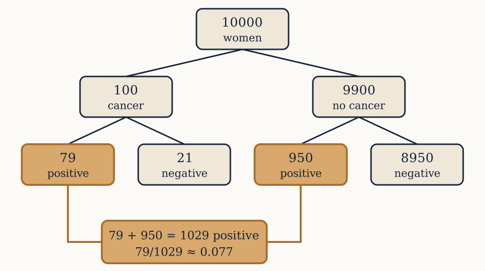
Take $10000$ women. About $100$ of them have cancer, and of those, $79$ test positive. The other $9900$ do not have cancer, and $950$ of them test positive anyway. So $79+950=1029$ women test positive in total, of whom $79$ have cancer:

the same answer, reached by dividing one count by another. The version with percentages hides the fact that the two groups being compared are of wildly different sizes; the version with counts puts the $9900$ on the page where it cannot be forgotten. When you want to sanity-check any Bayes calculation, do it this way, with a round population and whole people.

Odds and the weight of evidence

There is a form of the theorem in which the awkward denominator disappears. Write Bayes for $H$ and for $H^c$ with the same evidence and divide one by the other. The $P(E)$ cancels, leaving

In words: posterior odds equal prior odds times the likelihood ratio. Odds of $p$ against $1-p$ convert back to a probability by $p=\text{odds}/(1+\text{odds})$.

The likelihood ratio is the entire contribution of the evidence, and it is a property of the test alone, free of the base rate. For the mammogram it is $0.792/0.096=8.25$: a positive result multiplies the odds by $8.25$, whoever is tested and whatever they believed beforehand. That is the honest summary of what a test is worth, and it explains the earlier result at once. Prior odds of cancer are $1$ to $99$, or $0.0101$. Multiply by $8.25$ to get posterior odds of $0.0833$, and convert: $0.0833/1.0833\approx 0.0769$. Multiplying odds by $8.25$ sounds impressive and moves a probability of $0.01$ only to $0.077$, because odds far from one are hard to shift.

Repeated independent tests multiply their likelihood ratios, which makes sequential updating trivial. Two independent positive mammograms give odds $0.0101\times {8.25}^2=0.6875$, a probability of $0.4074$. Three give odds $5.672$ and a probability of $0.8501$. Note also that the order of the evidence never appears in the product, so updating on $E_1$ then $E_2$ gives exactly what updating on $E_2$ then $E_1$ gives, and both equal updating on both at once. A Bayesian cannot be led anywhere by the sequencing of the evidence, only by its content.

Example. A blood test has likelihood ratio $12$ for a positive result. A patient's prior probability of the condition is $0.05$. What is the posterior probability after one positive?

Prior odds are $0.05/0.95=0.05263$. Multiply by $12$ to get $0.6316$. Convert back: $0.6316/1.6316\approx 0.3871$, so about $39$ percent.

Now you. The same patient tests positive a second time, independently. What is the probability now?

Negative results and the other error

A test has two ways of being wrong, and the odds form handles the second as easily as the first. The likelihood ratio for a negative result is $P(-|H)/P(-|H^c)$, which for the mammogram is $(1-0.792)/(1-0.096)=0.208/0.904=0.2301$. A negative multiplies the odds by $0.23$, cutting them by more than a factor of four.

Starting from prior odds of $1$ to $99$, a negative mammogram gives odds $0.0101\times 0.2301=0.002324$, a probability of $0.002319$, down from $0.01$. So the test does useful work in both directions: it takes a one-in-a-hundred risk down to about one in four hundred and thirty. A likelihood ratio near $1$, in either direction, is the signature of a test not worth doing, since it leaves the odds where it found them.

Example. For the drug test above, what is the likelihood ratio of a negative result, and what does a negative do to an athlete whose prior probability of doping was $0.05$?

The ratio is $(1-0.99)/(1-0.02)=0.01/0.98=0.010204$. Prior odds $0.05/0.95=0.05263$, so posterior odds are $0.000537$ and the probability is $0.000537$, roughly one in $1863$.

Now you. A test has sensitivity $0.95$ and false positive rate $0.10$. What are its likelihood ratios for a positive and for a negative result?

What the theorem cannot give you

Bayes' theorem is a rule for revising a probability. It is not a rule for having one in the first place, and the prior has to come from somewhere outside it. In the mammography problem the prior was a measured population rate, which is uncontroversial. In a courtroom, or in assessing a scientific hypothesis, there is no population to count, and the prior is a judgement. Two honest people with different priors will reach different posteriors from the same evidence, and the theorem cannot arbitrate between them.

What it does guarantee is that they converge under enough evidence. Each new independent observation multiplies both people's odds by the same likelihood ratio, so a disagreement of a factor of a hundred in the prior is erased by evidence worth a factor of a hundred, and strong evidence swamps any prior that was not dogmatic. The exception is a prior of exactly $0$ or $1$, which multiplication can never move: certainty is not a strong opinion but an unreachable one, and this is the mathematical content of the advice to never be completely sure.

The theorem also silently assumes that the hypotheses listed are exhaustive. The denominator sums over the alternatives you thought of, so if the true explanation is not in the list, the posterior is confidently wrong. A high posterior means "best of what was considered", not "true".

So far every hypothesis and every event has been a yes-or-no affair. Most quantities of interest are not: how many defective items in a batch, how long until a component fails, how far a measurement is from its target. Attaching a number to each outcome, and asking what that number does on average, is the next step.

Everything so far has been about events, which either happen or do not. Most questions worth asking concern a quantity instead: how many defective items, how long a wait, how much money. This lesson attaches numbers to outcomes, defines the average of such a number, and proves one property of that average that does more work than any other result in the subject.

A number attached to every outcome

A random variable is a function from the sample space to the real numbers. It assigns to each outcome $\omega$ a value $X(\omega )$. That is all it is, and the name is doubly misleading: it is not random, being a fixed function, and it is not a variable, being a function. The randomness lives in which outcome occurs, and $X$ merely reports a number about it.

Roll two dice, so $\Omega$ is the $36$ ordered pairs, and let $X$ be the total. Then $X((3,4))=7$, and $X$ is defined on every outcome with no ambiguity. Once $X$ exists, statements about it become events in the old sense: "$X=7$" names the set of six pairs that total seven, and "$X\ge 10$" names a set of six pairs, so both have probabilities by the rules already established.

A variable taking values in a finite or countable set is discrete, which covers everything in this lesson and the next three. Its behaviour is captured completely by the probability mass function

which is non-negative and sums to $1$ over all possible values, since the events $\{X=x\}$ partition $\Omega$. For the two-dice total, the mass function runs $1/36,2/36,\dots ,6/36,\dots ,2/36,1/36$ across the values $2$ to $12$, and those eleven numbers sum to $36/36$.

The mass function throws away the sample space, and that is its point. Two completely different experiments with the same mass function are interchangeable for every purpose that mentions only $X$. From here on the underlying $\Omega$ is rarely written down.

The average of a random variable

Suppose the experiment is repeated $N$ times and $X$ takes the value $x$ on about $Np(x)$ of them. The arithmetic mean of the observed values is then

with $N$ cancelling. That expression is taken as the definition of the expectation, also called the expected value or the mean:

It is a weighted average of the possible values, weighted by their probabilities, and it is a fixed number, not a random one. Whether the long-run average really converges to it is a theorem proved much later in this course, not an assumption made here.

For a single fair die, $E[X]=(1+2+3+4+5+6)/6=3.5$, a value the die can never show. Expectation is a centre of mass, not a prediction, and reading it as "what will happen" is the first of several ways it misleads. For the two-dice total, $E[X]=7$, which the sum can show, and which sits at the centre of the symmetric mass function.

Example. A European roulette wheel has $37$ pockets: $18$ red, $18$ black and one green zero. You stake $1$ unit on red, winning $1$ if red comes up and losing your stake otherwise. What is the expected gain per spin?

so the house keeps about $2.7$ percent of everything staked, on average, whatever the bet.

Now you. An American wheel has $38$ pockets, with both a zero and a double zero, so $18$ are red. What is the expected gain per unit staked on red?

Functions of a random variable

If $X$ is a random variable then so is $g(X)$ for any function $g$, since a function of a function is a function. Its expectation could be found by first working out the mass function of $g(X)$, and it never has to be, because

The proof is a regrouping: gather the outcomes according to the value of $X$ rather than the value of $g(X)$, and every outcome is still counted exactly once with its own probability. The result is often called the law of the unconscious statistician, from the habit of using it without noticing that it needs proof.

Two consequences are worth having on hand. First, $E[aX+b]=aE[X]+b$ for constants $a$ and $b$, since the sum splits and $\sum _{x}p(x)=1$. Expectation moves through a change of units unharmed: a temperature in Fahrenheit has $9/5$ times the expected Celsius value plus $32$. Second, $E[X^2]$ is generally not $(E[X]{)}^2$. For a fair die, $E[X^2]=(1+4+9+16+25+36)/6=91/6\approx 15.1667$, while $(E[X]{)}^2=12.25$. The gap of $2.9167$ is not an error; the next lesson identifies it as the variance.

The practical consequence is that a payout must be averaged after the function is applied, never before. A stall charging $2$ units to roll a die and paying out the square of the result takes in $2$ and pays out $E[X^2]\approx 15.1667$, losing about $13.17$ units a play; pricing it from $(E[X]{)}^2=12.25$, or worse from $E[X]=3.5$, would have hidden that.

Linearity, which asks for nothing

Here is the result that earns its keep. For any random variables $X$ and $Y$ defined on the same sample space,

The proof works outcome by outcome rather than value by value. Writing the expectation as a sum over $\Omega$,

which is nothing but the associativity of addition. Notice what is absent: no independence, no assumption about how $X$ and $Y$ relate, not even that they are different quantities. It holds when $Y=X$, when $Y=-X$, when $Y$ is a deliberately hostile function of $X$. Extended to any finite number of terms it says the expectation of a sum is always the sum of the expectations.

This is stronger than it looks, because most quantities of interest are sums of simple pieces whose joint behaviour is a nightmare and whose individual behaviour is trivial. The two-dice total illustrates the pattern in miniature: rather than summing $\sum _{x}xp(x)$ over the eleven values with their awkward weights, write $X=X_1+X_2$ and get $3.5+3.5=7$ immediately.

Example. Five cards are dealt from a shuffled deck. What is the expected number of hearts?

Let $X_i$ be $1$ if the card in position $i$ is a heart and $0$ otherwise, so the number of hearts is $X_1+\cdots +X_5$. Each individual card is equally likely to be any of the $52$, so $E[X_i]=P(\text{heart})=13/52=0.25$. Linearity gives $5\times 0.25=1.25$ hearts expected. The cards are emphatically not independent, since dealing a heart makes the next heart less likely, and linearity does not care.

Now you. Ten cards are dealt from the same deck. What is the expected number of aces?

Indicators, and the problems they crack

The technique in that example deserves a name. An indicator variable $I_A$ takes the value $1$ when the event $A$ occurs and $0$ when it does not, and its expectation is

so expectation and probability are the same operation on indicators. Any count is a sum of indicators, one per thing that might be counted, and by linearity its expectation is the sum of the separate probabilities. Nothing about dependence ever enters.

Take the classic: $n$ letters are put at random into $n$ addressed envelopes. How many arrive at the right address? The exact distribution of the number of matches is a genuinely awkward object involving alternating sums. Its mean is not. Let $I_i$ indicate that letter $i$ is in its own envelope. Any given letter is equally likely to be in any of the $n$ envelopes, so $E[I_i]=1/n$, and the expected number of matches is $n\times (1/n)=1$ for every $n$. One letter arrives correctly on average, whether there are ten letters or ten million.

Or the coupon collector. There are $n$ different coupons, one at random in each packet. Let $T_k$ be the number of packets bought while holding exactly $k$ distinct coupons. Each purchase in that stretch is new with probability $(n-k)/n$, and a wait for a success with constant probability $p$ has expectation $1/p$, proved in the lesson on the binomial family. So $E[T_k]=n/(n-k)$, and the total is

For $n=6$, a full set of six needs $6\times 2.45=14.7$ packets on average, and for $n=50$ it is $225$. Collecting the last few is most of the work: the final coupon alone takes $n$ packets on average.

Example. A fair die is rolled six times. What is the expected number of distinct faces seen?

Let $I_f$ indicate that face $f$ appears at least once. It fails to appear with probability $(5/6{)}^6\approx 0.3349$, so $E[I_f]\approx 0.6651$. Summing over the six faces gives $6\times 0.6651\approx 3.99$ distinct faces, about four.

Now you. A fair coin is tossed $10$ times. What is the expected number of tosses that match the toss before them, out of the $9$ adjacent pairs?

Where the mean is not enough

Expectation compresses a whole distribution into one number, and the compression discards things that matter.

Consider two propositions. The first pays $1$ unit with certainty. The second pays $1000000$ units with probability ${10}^{-6}$ and nothing otherwise. Both have expectation exactly $1$, and nobody treats them as equivalent. Expectation cannot distinguish a certainty from a lottery, because it never asks how far the outcomes stray from their average.

The extreme case was posed by Nicolas Bernoulli in 1713. A coin is tossed until it lands heads; if this takes $n$ tosses, the payout is $2^n$ units. The probability of stopping at toss $n$ is $2^{-n}$, so each term of the expectation contributes $2^{-n}\times 2^n=1$, and the sum over infinitely many terms diverges. The expected payout is infinite, and no one will pay even $100$ units to play, since a payout above $100$ requires at least seven tosses, which happens with probability $2^{-6}=0.015625$, about once in $64$ plays. Daniel Bernoulli's 1738 resolution, that people value money by something growing more slowly than the amount, launched utility theory, but the plain mathematical point stands on its own: an expectation can exist and be useless, or fail to exist while the variable is perfectly well behaved.

What is missing is a measure of how widely the values are spread around the mean. Building one, discovering that it adds when expectations of products do not, and extracting a guarantee about how far from the mean a variable can stray, is the next lesson.

Expectation compresses a distribution to a single number and cannot tell a certainty from a lottery with the same average. This lesson builds the second number, the one that measures spread, and finds that it has a property expectation does not share and a consequence expectation cannot deliver.

Choosing a measure of spread

Spread means typical distance from the centre, so the obvious candidate is the mean of $X-\mu$, writing $\mu =E[X]$ throughout. That candidate dies immediately: $E[X-\mu ]=E[X]-\mu =0$ for every variable whatsoever, since the deviations above and below the mean cancel exactly. Any usable measure has to remove the signs first.

Two ways to do it. Take absolute values, giving the mean absolute deviation $E|X-\mu |$, or take squares, giving $E[(X-\mu {)}^2]$. The absolute version is the more natural reading of "typical distance" and is almost never used, for reasons that are practical rather than deep. The absolute value has no derivative at zero and does not expand when a sum is substituted into it, so a formula containing it usually stays stuck. The square expands, and it is that expansion, three lines below, that produces the additivity the whole subject runs on.

So define the variance

and, because squaring changed the units, the standard deviation $\sigma =\sqrt{\mathrm{operatorname}\{Var}(X)\}$, which is back in the units of $X$ and is the number to quote. A variance is never negative, since it averages squares, and it is zero exactly when $X$ equals $\mu$ with probability one.

Expanding the square gives a version that is easier to compute:

so the variance is the mean of the square minus the square of the mean, and the gap noticed in the previous lesson between $E[X^2]=91/6$ and $(E[X]{)}^2=12.25$ for a fair die is exactly its variance: $35/12\approx 2.9167$, with $\sigma \approx 1.7078$.

What scaling does

Shifting a variable moves its mean and leaves its spread alone; stretching it stretches the spread. Both facts follow from the definition. For constants $a$ and $b$, the variable $aX+b$ has mean $a\mu +b$, so its deviation from its own mean is $a(X-\mu )$, and squaring introduces $a^2$:

The additive constant vanishes entirely, which is right: adding ten to every value moves the whole distribution without spreading it. The factor $a^2$ rather than $a$ is the price of working with squares, and the standard deviation, taking the square root, scales the sensible way.

This licenses standardisation. Given any $X$ with mean $\mu$ and standard deviation $\sigma >0$, the variable

has mean $0$ and variance $1$, since the shift kills the mean and the division by $\sigma$ divides the variance by ${\sigma }^2$. A value of $Z$ counts how many standard deviations $X$ is from its mean, and it is dimensionless, so heights and test scores and share prices become comparable. This construction returns in the lesson on the normal curve, where it does most of the work.

A quick check on the rule: a game paying $10X+5$ units on a roll of a fair die has mean $10(3.5)+5=40$ units and standard deviation $10\times 1.7078=17.078$ units, the additive $5$ contributing nothing to the spread and everything to the centre.

Why variances add

Expectation adds unconditionally. Variance does not, and the exact condition is worth deriving. Let $X$ and $Y$ have means ${\mu }_X$ and ${\mu }_Y$. Then

by expanding the square inside the expectation and using linearity on the three resulting terms. The last piece is the covariance

which is positive when the two tend to be above their means together, negative when one being high goes with the other being low, and zero when there is no such tendency on average.

If $X$ and $Y$ are independent then $E[XY]=E[X]E[Y]$, because the joint mass function factorises and the double sum splits into a product of two sums. So independence forces the covariance to zero and leaves

Two cautions. First, the implication runs one way only: zero covariance does not imply independence. Let $X$ be $-1$, $0$ or $1$ with probability $1/3$ each and $Y=X^2$. Then $E[XY]=E[X^3]=0=E[X]E[Y]$, so the covariance vanishes, yet $Y$ is a function of $X$ and could hardly be more dependent. Covariance detects linear association and is blind to the rest.

Second, dependence can cancel spread entirely. Let $Y=7-X$ for a die roll $X$. Both have variance $35/12$, and their sum is the constant $7$, whose variance is zero. Here the covariance is $-35/12$ and exactly cancels the two positive terms. Assuming variances add when the variables are linked is how a portfolio of correlated assets comes to look far safer than it is.

Example. Two fair dice are rolled independently. What are the variance and standard deviation of the total?

Each die has variance $35/12$, and independence lets them add: $\mathrm{operatorname}\{Var\}=70/12\approx 5.8333$, so $\sigma \approx 2.4152$. The mean is $7$, so a total is typically about two and a half away from seven.

Now you. Three independent fair dice are rolled. Find the variance and standard deviation of the total.

The square root of n

Now take $n$ independent copies of the same variable, each with mean $\mu$ and variance ${\sigma }^2$: repeated measurements, repeated bets, repeated trials. Their sum $S_n$ has mean $n\mu$ by linearity and variance $n{\sigma }^2$ by additivity, so

The sum's spread grows, but only as the square root of the number of terms, while its mean grows as $n$ itself. Divide through to get the average ${\bar{X}}_n=S_n/n$, which by the scaling rule has variance $n{\sigma }^2/n^2={\sigma }^2/n$ and therefore

This single formula is why measurements are repeated. Averaging four readings halves the spread, twenty-five readings divides it by five, ten thousand readings by a hundred. It is also a warning about cost: each further factor of two in precision costs four times the data, so precision gets expensive fast.

It also explains the two columns of Kerrich's coin table from the first lesson. The number of heads in $n$ tosses has standard deviation $\sqrt{n}/2$, which grows without bound, so the absolute surplus of heads drifts further from zero. The fraction of heads has standard deviation $1/(2\sqrt{n})$, which shrinks to nothing. Both columns behave exactly as they must, and neither is evidence about the coin.

Example. A measurement has standard deviation $0.8$ grams. How many independent repeats are needed for the average to have a standard deviation of $0.1$ grams?

Set $0.8/\sqrt{n}=0.1$, so $\sqrt{n}=8$ and $n=64$ measurements. Halving that target again, to $0.05$ grams, would take $256$.

Now you. An opinion poll of $1000$ people estimates a proportion whose standard deviation is at most $0.5/\sqrt{n}$. What is that bound for $n=1000$, and how many people would be needed to halve it?

Chebyshev's guarantee

Variance is more than a descriptive number: it bounds how much probability can sit far from the mean, for any distribution at all. Take any $k>0$ and let $A$ be the event $|X-\mu |\ge k\sigma$. Then

The first inequality drops the contribution from outcomes outside $A$, which is non-negative. The second replaces $(X-\mu {)}^2$ by its minimum value on $A$, which is $k^2{\sigma }^2$ by the definition of $A$. Dividing by $k^2{\sigma }^2$ gives Chebyshev's inequality, published by Pafnuty Chebyshev in 1867:

No distribution can put more than a quarter of its probability two or more standard deviations from its mean, and never more than a ninth beyond three, whatever shape it has: no symmetry assumed, no bell curve, nothing but a finite variance.

The bound is very loose in practice, and deliberately so, since it must cover the worst case. Toss a fair coin $100$ times: the number of heads has mean $50$ and standard deviation $5$, so Chebyshev caps $P(|X-50|\ge 15)$ at $1/9\approx 0.1111$. The true value, computable exactly from the binomial formula of the next lesson, is $0.00352$, smaller by a factor of thirty. Chebyshev is not for computing probabilities. It is for proving that they must be small, which is exactly what is needed to prove the law of large numbers later in this course.

Example. A production line fills bags with mean $500$ grams and standard deviation $8$ grams. What does Chebyshev guarantee about the fraction of bags between $480$ and $520$ grams?

The interval is $\mu \pm 20$ grams, which is $k=20/8=2.5$ standard deviations. Chebyshev bounds the outside at $1/{2.5}^2=0.16$, so at least $84$ percent of bags lie inside. If the weights happen to follow a normal curve the real figure is above $98$ percent, and the guarantee holds whether or not they do.

Now you. For the same line, what fraction of bags does Chebyshev guarantee lie between $476$ and $524$ grams?

What two numbers still miss

Mean and variance now exist for any variable with a finite second moment, they behave predictably under scaling, they add under independence, and they yield a universal tail bound. That is enough to say something about every distribution and not enough to say much about any particular one.

Two distributions can share a mean and a variance and look nothing alike. Symmetric and skewed, single-peaked and twin-peaked, bounded and unbounded: none of that is visible in the first two moments. Worse, some distributions have no finite variance at all, and for those Chebyshev says nothing and the square root of $n$ law fails outright. Such heavy-tailed cases are not exotic curiosities; they appear in insurance losses and in financial returns, where a model chosen for its convenient variance quietly understates the risk of the events that matter.

The productive move is to stop treating distributions one at a time. A handful of mechanisms generate most of the distributions that occur, and each mechanism fixes the whole mass function, with the mean and variance falling out of it. The first and most important of those mechanisms is repeated independent trials with a fixed success probability, and it is the next lesson.

A distribution earns a name when one mechanism produces it over and over, and the commonest mechanism of all is a fixed number of independent attempts at the same thing. This lesson derives what that produces, tests it against a dice experiment run in 1894, and finds the regime where the formula stops being usable.

One trial, two outcomes

Start with the smallest case. A Bernoulli trial is an experiment with two outcomes, labelled success and failure, with $P(\text{success})=p$. Its indicator $X$ takes the value $1$ or $0$, and everything about it follows from the previous two lessons:

so $\mathrm{operatorname}\{Var\}(X)=p-p^2=p(1-p)$. That variance is worth a moment. It is zero at $p=0$ and at $p=1$, where the outcome is certain and there is nothing to vary, and it is largest at $p=0.5$, where it equals $0.25$. Maximum uncertainty sits at even odds, which matches intuition and is here a consequence rather than an assertion. Writing $q=1-p$ for the failure probability, the variance is $pq$.

The name is Jacob Bernoulli's, from Ars Conjectandi, written before his death in 1705 and published in 1713, which is also where the first law of large numbers appears.

Counting successes

Now run $n$ such trials, independently, with the same $p$ each time, and let $X$ be the number of successes. Any particular sequence with $k$ successes and $n-k$ failures has probability $p^k{q}^{n-k}$ by independence, and this does not depend on the order in which the successes fell. So the probability of $k$ successes is that quantity times the number of sequences that have $k$ successes, which is the number of ways to choose which trials succeeded:

This is the binomial distribution, written $X\sim \text{Bin}(n,p)$, and both ingredients came from earlier lessons: the counting of positions from the combinations lesson, the multiplication of probabilities from independence. The masses sum to $1$ because the right-hand side is the general term of the binomial theorem applied to $(p+q{)}^n=1^n=1$, which is where the name comes from.

Toss a fair coin ten times. The probability of exactly three heads is $C(10,3)(0.5{)}^{10}=120/1024\approx 0.1172$, and the probability of eight or more is $(45+10+1)/1024=56/1024\approx 0.0547$. That last figure is worth remembering: getting eight or more heads out of ten is not rare enough to prove anything about a coin.

Three conditions are being assumed, and each fails somewhere real. The number of trials is fixed in advance, so stopping when you like invalidates the formula. The trials are independent, which fails for cards dealt without replacement. And $p$ is the same throughout, which fails when a machine drifts as it heats up.

Example. A machine produces items with a $5$ percent defect rate, independently. In a box of $20$, what is the probability of no defects, and of two or more?

$P(0)={0.95}^{20}\approx 0.3585$. $P(1)=20(0.05)(0.95{)}^{19}\approx 0.3774$. So $P(\ge 2)=1-0.3585-0.3774\approx 0.2642$. More than a quarter of boxes carry at least two defects, even though the expected number is only $1$.

Now you. For the same machine, what is the probability that a box of $10$ contains no defects?

Mean and variance without a single sum

The direct route to $E[X]$ is $\sum _{k}kC(n,k)p^k{q}^{n-k}$, which can be done and is unpleasant. The indicator route is two lines.

Write $X=I_1+I_2+\cdots +I_n$, where $I_j$ indicates success on trial $j$. Linearity of expectation, which needs nothing at all, gives

Independence lets the variances add too, and each contributes $pq$:

Ten fair tosses have mean $5$ and standard deviation $\sqrt{10\times 0.25}\approx 1.58$. The box of twenty items has mean $1$ and standard deviation $\sqrt{20(0.05)(0.95)}\approx 0.9747$.

The shape follows from the ratio of consecutive masses,

which decreases as $k$ grows, so the masses rise while that ratio exceeds $1$ and fall afterwards. The distribution therefore has a single peak, located at $k=\lfloor (n+1)p\rfloor$, close to the mean $np$ as it should be. At $p=0.5$ the mass function is symmetric, since swapping successes for failures leaves it unchanged, and away from $0.5$ it is skewed towards the boundary it is furthest from.

Weldon's twenty-six thousand throws

In 1894 Raphael Weldon threw twelve dice together, over and over, and recorded how many showed a five or a six. He did this $26306$ times, which is $315672$ individual dice rolls, and sent the tally to Karl Pearson. On fair dice the probability of a five or six is $1/3$, so each throw of twelve should give $\text{Bin}(12,1/3)$, with mean $4$ successes.

The observed total was $106602$ successes, an average of $4.0524$ per throw, giving $\hat{p}=106602/315672\approx 0.33771$ against the theoretical $0.33333$. The excess looks tiny. Ask whether it could be chance, using the machinery just built: if $p$ were exactly $1/3$, the total number of successes would have mean $315672/3=105224$ and standard deviation $\sqrt{315672\times \frac{13}{\times }\frac{23}{\}}\approx 264.9}$. The observed total is $1378$ above the mean, which is $5.2$ standard deviations out. Chebyshev alone caps that at $1/{5.2}^2\approx 0.037$, and the true figure is vastly smaller.

So the dice were not fair, and the reason is manufacturing: the pips are drilled into the faces, removing material, so the six face is lightest and lands uppermost slightly more often than a third of the time. This is what a probability model earns its keep by doing. A model precise enough to be wrong turned a $0.4$ percentage point discrepancy, invisible to any player, into a definite statement about how dice are made.

Example. A drug is claimed to be no better than a coin toss at curing a condition. In a trial of $8$ patients it cures $7$. Under the coin-toss hypothesis, how likely is a result this extreme or more?

$P(X\ge 7)=(C(8,7)+C(8,8))/2^8=(8+1)/256\approx 0.0352$. About one trial in twenty-eight would do this well by luck alone, which is suggestive and thin, and it is why trials are not run on eight patients.