Linear Algebra

Solving two equations in two unknowns is school algebra, and solving two thousand equations in two thousand unknowns is a different activity entirely, which is what this subject exists to make possible.

This course assumes the material of Mathematical Foundations: manipulating algebraic expressions, functions and their graphs, coordinates in the plane, and enough trigonometry to read $\cos \theta$ and $\sin \theta$ off a unit circle. Nothing else is assumed. In particular, calculus is never used, and where a connection to it exists it is signposted and skippable.

What makes an equation linear

An equation is linear in the unknowns $x_1,x_2,\dots ,x_n$ when it can be written as

with the coefficients $a_i$ and the constant $b$ being fixed numbers. Every unknown appears to the first power, alone, multiplied only by a number. That rules out $x^2$, it rules out $xy$, and it rules out $\sin x$, $1/x$ and $\sqrt{x}$. Note that $3x+4y=12$ qualifies, and so does $0x+0y=0$, and so does $7x_1-2x_2+0x_3=-1$, where the missing unknown is present with coefficient zero.

This looks like a severe restriction, and it is worth being clear that it is one. Most equations that describe the world are not linear. What makes the restricted class worth an entire subject is a combination of three facts. Linear systems can actually be solved, exactly, by a procedure that always terminates. Many genuinely non-linear problems are linear when examined closely enough, which is why a bridge deflecting slightly under load, a circuit at small signal, and a chemical mixture at low concentration are all handled linearly. And problems that are hopelessly non-linear are usually attacked by solving a linear system repeatedly, which is what Newton's method, every finite element package and every step of training a neural network are doing underneath.

A system of linear equations is several of them at once, sharing their unknowns. A solution is an assignment of numbers to the unknowns that satisfies every equation simultaneously, not merely one of them. The entire difficulty is that word: simultaneously.

Two unknowns, and two lines

With two unknowns the whole situation is visible. The equation $2x+3y=7$ is satisfied by infinitely many pairs $(x,y)$, and plotted in the plane they form a straight line, which is why the equations are called linear in the first place. A second equation gives a second line. A solution of the system is a point on both lines, so solving the system means intersecting them.

Two distinct lines in a plane intersect in exactly one point unless they are parallel, in which case they meet nowhere, unless they are the same line, in which case they meet everywhere along it. Those are the only three possibilities, and no fourth case exists: two lines cannot meet in exactly two points. That fact is worth holding on to, because it survives intact into two thousand dimensions where nothing can be drawn.

Example. Solve $2x+3y=7$ and $4x-y=7$.

Multiply the second equation by $3$ to get $12x-3y=21$, and add it to the first, so that the $y$ terms cancel: $14x=28$, giving $x=2$. Substituting back into the second equation, $8-y=7$, so $y=1$. Check both original equations: $2(2)+3(1)=7$ and $4(2)-1=7$. The lines cross at $(2,1)$.

Now you. Solve $3x+2y=16$ and $x-y=2$.

Elimination

The method in that example, adding a multiple of one equation to another so that an unknown vanishes, is the whole of it. Scaled up and made systematic it is called Gaussian elimination, though it appears in the Chinese Nine Chapters on the Mathematical Art around two thousand years before Gauss, worked with counting rods on a board.

Three operations are permitted, and each is reversible, which is what guarantees that they never gain or lose a solution. Any equation may be multiplied by a non-zero number. Any multiple of one equation may be added to another. Any two equations may be swapped. The goal is to reach a triangular form, in which the first equation involves all the unknowns, the second has lost the first unknown, the third has lost the first two, and so on down, at which point the last equation contains one unknown and the rest fall out by back substitution.

Take a system of three:

Use the first equation to remove $x$ from the other two. Adding $1.5$ times the first to the second gives $0x+0.5y+0.5z=1$. Adding the first to the third gives $0x+2y+z=5$. The first unknown is now confined to the first equation.

Now use the new second equation to remove $y$ from the third. Subtracting $4$ times $(0.5y+0.5z=1)$ from $(2y+z=5)$ gives $0y-z=1$, so $z=-1$.

Back substitute. From $0.5y+0.5z=1$ with $z=-1$: $0.5y=1.5$, so $y=3$. From the first equation, $2x+3-(-1)=8$, so $2x=4$ and $x=2$. The solution is $(2,3,-1)$, and substituting it into all three original equations gives $8$, $-11$ and $-3$ as required.

Two features of that calculation matter more than the answer. It was mechanical: at no point was ingenuity required, only a decision about which equation to use to clear which unknown. And it terminated: there is no possibility of the procedure wandering, because each step permanently removes one unknown from one equation and the supply of both is finite.

Example. Solve $x+2y+z=6$, $2x+y-z=1$ and $x-y+2z=5$ by elimination.

Subtract $2$ times the first from the second: $-3y-3z=-11$. Subtract the first from the third: $-3y+z=-1$. Now subtract the second of these from the third: $4z=10$, so $z=2.5$. Then $-3y=-1-z=-3.5$, so $y=7/6\approx 1.1667$, and $x=6-2y-z=6-2.3333-2.5=1.1667$. Check the second equation: $2(1.1667)+1.1667-2.5=1.0$, as required.

Now you. Solve $x+y+z=6$, $2y+5z=-4$ and $2x+5y-z=27$.

The three outcomes

Elimination cannot fail, but it can end somewhere other than a triangle, and there are exactly two ways for that to happen.

Take $x+2y=4$ and $2x+4y=7$. Subtracting twice the first from the second gives $0x+0y=-1$, which no assignment of $x$ and $y$ can satisfy. The system is inconsistent and has no solution. Geometrically the two lines have the same slope and different intercepts: they are parallel, and never meet.

Now change one digit: $x+2y=4$ and $2x+4y=8$. The same step gives $0x+0y=0$, which every pair satisfies. The second equation was the first one in disguise, carrying no information, and the system is left with one genuine equation in two unknowns. Setting $y$ to any value $t$ gives $x=4-2t$, so the solutions form a whole line: $(4,0)$, $(2,1)$, $(0,2)$ and infinitely many more. The system is underdetermined.

So a linear system has no solution, exactly one, or infinitely many. It can never have exactly two, or exactly seventeen. The reason is easy to see and worth seeing now: if $\mathbf{p}$ and $\mathbf{q}$ are both solutions then so is every point on the line joining them, because averaging two solutions of $a_1{x}_1+\cdots +a_n{x}_n=b$ in any weighted way that sums to one gives $b$ again. Two solutions therefore drag a continuum in with them. Later lessons make this precise, and give the solution set a name and a dimension.

Example. Classify $3x-6y=9$ and $-x+2y=-3$.

Add $3$ times the second to the first: $0=0$. The second equation is $-1/3$ times the first, so there is one genuine equation, $x-2y=3$, and infinitely many solutions: $x=3+2t$, $y=t$. Two of them are $(3,0)$ and $(5,1)$, and both satisfy the original pair.

Now you. Classify $4x-2y=5$ and $-6x+3y=1$.

What it costs

The reason a subject is needed rather than a technique is that $n$ grows. Clearing the first unknown from $n-1$ equations of $n+1$ numbers each costs roughly $n^2$ multiplications, and repeating for each unknown in turn totals about $n^3/3$ multiplications and as many additions. For $n=1000$ that is $3.3\times {10}^8$ operations, a fraction of a second on any laptop. For $n=5000$ it is $4.2\times {10}^{10}$, about forty seconds at a billion operations per second. For $n={10}^6$, the size of system a serious engineering simulation produces, it is $3.3\times {10}^{17}$, which is out of reach by brute force and is solved instead by methods that exploit the structure of the particular matrix, most of whose entries are zero.

Compare the alternative that school sometimes teaches for small systems, Cramer's rule, which expresses each unknown as a ratio of determinants. Computing an $n$ by $n$ determinant by the naive expansion costs about $n!$ multiplications. For $n=20$ that is $2.4\times {10}^{18}$ operations, seventy-seven years at a billion per second, against $2700$ operations for elimination. Cramer's rule is a theoretical statement, not an algorithm, and this course will treat it as one.

Example. Roughly how many multiplications does elimination need for $n=200$, and how does that compare with $n=2000$?

Using $n^3/3$: for $n=200$ it is $8\times {10}^6/3=2.7\times {10}^6$. For $n=2000$ it is $8\times {10}^9/3=2.7\times {10}^9$. Ten times the unknowns costs a thousand times the work, because the count is cubic.

Now you. A solver manages $2\times {10}^9$ multiplications per second. Roughly how long does it take on a system with $n=5000$?

The unknowns were never used

Look back at the elimination worked above and ask which symbols did any work. The letters $x$, $y$ and $z$ were carried through every line and never once entered a calculation. All the arithmetic happened to the coefficients, and the letters were placeholders keeping the columns aligned. Written without them, the first system is nothing but a rectangle of numbers, with rows $(2,1,-1)$, $(-3,-1,2)$ and $(-2,1,2)$, together with the right hand side $(8,-11,-3)$.

That rectangle is a matrix, and the course to come is largely about taking it seriously as an object in its own right rather than as shorthand for a system. Two conventions are fixed now and used for the rest of the subject. A vector is a column of numbers, written in round brackets as $(8,-11,-3)$. A matrix is written as the list of its columns, so $A=[(2,-3,-2),(1,-1,1),(-1,2,2)]$ is the coefficient matrix of that system, whose first column collects the coefficients of $x$ from all three equations. When elimination needs to talk about a row it will say so explicitly.

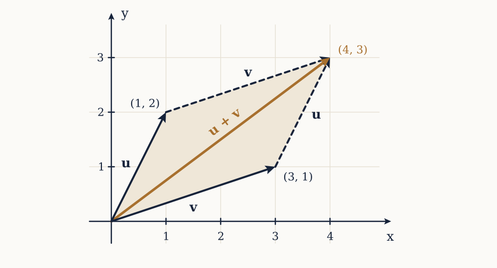
Writing the system by columns exposes something the row form hides. The three equations, taken together, say precisely that

where the multiplications and additions happen component by component. Solving is therefore asking what amounts of the three column vectors, added together, produce the target vector. That reading is the door into the geometry, and it turns the three outcomes above into three pictures rather than three algebraic accidents.

Honest limits

Exact arithmetic makes elimination flawless, and computers do not have exact arithmetic. If a pivot, the coefficient being divided by, is very small, dividing by it magnifies whatever rounding error the entry already carried, and the answer can come out wrong in every digit while the procedure reports no difficulty. The standard defence is partial pivoting: before clearing a column, swap in the row whose entry in that column is largest in absolute value. This costs almost nothing and, as James Wilkinson established in his backward error analysis around 1961, makes elimination reliable in practice, though contrived matrices that defeat it do exist. Every numerical library performs the swap by default.

There is also a limit worth naming at the start. Everything in this subject is exact and complete for the linear class, and the class really is a restriction. Nothing here will solve $x^2+y^2=1$. What the subject offers in exchange is that within its class, questions have answers and the answers can be computed and checked.

The next lesson takes up the column vectors that the coefficient matrix turned out to consist of, and asks what they are and what can be done to them.

A column of numbers can be read as an arrow in space, and the two readings support exactly the same arithmetic, which is what makes the geometry of the previous lesson available to systems of any size.

The previous lesson ended by writing a system of three equations as a statement about three columns of coefficients, $x(2,-3,-2)+y(1,-1,1)+z(-1,2,2)=(8,-11,-3)$. Two things happened to those columns there: they were multiplied by numbers, and they were added. This lesson takes those two operations as the definition of the objects, and then shows that measurement, length and angle and perpendicularity, comes from one further product that is not part of the definition at all.

An arrow and a list

A vector in the plane can be pictured as an arrow with a length and a direction, and represented by the pair of numbers saying how far it goes across and how far up: $(3,4)$ is three to the right and four up. The arrow is not anchored anywhere. An arrow from $(1,1)$ to $(4,5)$ and an arrow from the origin to $(3,4)$ are the same vector, because both are three across and four up, and it is convenient to draw every vector from the origin so that vectors and points can be identified.

In three dimensions the same works with triples, and beyond three the picture stops but the arithmetic does not. A vector in ${\mathbb{R}}^n$ is an ordered list of $n$ real numbers, and $n$ can be a million. This is not an abstraction for its own sake. A greyscale image of 1000 by 1000 pixels is a vector in ${\mathbb{R}}^{1000000}$, one coordinate per pixel. A month of daily closing prices for thirty stocks is a vector in ${\mathbb{R}}^{900}$. The word "direction" is unvisualisable in those spaces and remains perfectly well defined.

Two vectors are equal when every component matches. The zero vector $\mathbf{0}$ has every component zero, and it is the one vector with no direction. Vectors are written in bold, $\mathbf{v}$, and their components with subscripts, so $\mathbf{v}=(v_1,v_2,\dots ,v_n)$. Throughout this course a vector written in round brackets is a column, which matters from the lesson on matrices onward.

Two operations, and only two

Addition works component by component: $(1,2)+(3,1)=(4,3)$. Geometrically it is tip to tail. Draw the first arrow, start the second where the first ended, and the sum runs from the original start to the final tip. Equivalently, complete the parallelogram with the two arrows as sides and take its diagonal. That the two constructions agree is the statement that $\mathbf{u}+\mathbf{v}=\mathbf{v}+\mathbf{u}$, which is obvious from the components and not obvious from the picture.

Scalar multiplication multiplies every component by a number: $2(1,2)=(2,4)$ and $-0.5(4,3)=(-2,-1.5)$. The number is called a scalar to distinguish it from a vector. Geometrically, multiplying by $c$ stretches the arrow by a factor $|c|$, and reverses it when $c$ is negative. All the scalar multiples of one non-zero vector, taken together, form an infinite straight line through the origin.

Subtraction is not a third operation, being $\mathbf{u}+(-1)\mathbf{v}$, and it is worth reading geometrically: $\mathbf{u}-\mathbf{v}$ is the arrow from the tip of $\mathbf{v}$ to the tip of $\mathbf{u}$. That reading is used constantly, because the vector between two points is the difference of their position vectors.

There is deliberately no multiplication of two vectors in this list, and no division at all. The reason is that the operations are chosen to be exactly those that a system of linear equations performs, and the definition is worth stating in that spirit: a vector space is any set on which addition and scalar multiplication are defined and obey eight rules, that addition is commutative and associative, that a zero exists and each element has a negative, that scaling distributes over both kinds of sum, that $(cd)\mathbf{v}=c(d\mathbf{v})$, and that $1\mathbf{v}=\mathbf{v}$. Lists of $n$ numbers satisfy them. So do polynomials of degree at most five, which can be added and scaled and form a space of a size worked out two lessons from now. So do all real-valued functions on an interval, and so do the solutions of a differential equation like $y^{\prime \prime }+y=0$. Every result in this course rests on the eight rules alone, so every result applies to all of those, which is the return on the abstraction.

Example. With $\mathbf{u}=(2,-1,3)$ and $\mathbf{v}=(1,4,-2)$, compute $3\mathbf{u}-2\mathbf{v}$.

Scale first: $3\mathbf{u}=(6,-3,9)$ and $2\mathbf{v}=(2,8,-4)$. Subtract component by component: $(6-2,-3-8,9+4)=(4,-11,13)$.

Now you. With the same $\mathbf{u}$ and $\mathbf{v}$, compute $\mathbf{u}+2\mathbf{v}$ and check that it equals $(4,7,-1)$.

Length

Nothing said so far measures anything. Length has to be added, and in the plane Pythagoras supplies it: the arrow $(3,4)$ is the hypotenuse of a right triangle with legs $3$ and $4$, so its length is $\sqrt{9+16}=5$. In three dimensions apply Pythagoras twice, once in the base plane and once vertically, giving $\sqrt{v_1^2+v_2^2+v_3^2}$. The vector $(1,2,2)$ has length $\sqrt{1+4+4}=3$ exactly.

In $n$ dimensions the same formula is taken as the definition, since there is no triangle to appeal to:

The double bars distinguish it from the absolute value of a number, which it generalises. Length is never negative, and is zero only for the zero vector. Scaling behaves as the picture demands: $\Vert c\mathbf{v}\Vert =|c|\Vert \mathbf{v}\Vert$, because every component is multiplied by $c$ and every square by $c^2$.

A vector of length one is a unit vector, and dividing any non-zero vector by its own length produces one pointing the same way, an operation called normalising. This separates a vector into a direction and a magnitude, which is what makes it useful.

Example. Find the length of $(5,-12)$ and the unit vector in its direction.

$\Vert (5,-12)\Vert =\sqrt{25+144}=\sqrt{169}=13$. Dividing gives $(5/13,-12/13)=(0.3846,-0.9231)$, and as a check ${0.3846}^2+{0.9231}^2=0.1479+0.8521=1.0000$.

Now you. Find the length of $(2,3,6)$ and normalise it.

The dot product

Angles need one more construction, and it is the single most useful formula in the subject. The dot product of two vectors with the same number of components multiplies them componentwise and adds the results:

The output is a number, not a vector, which is why it is also called the scalar product. For $(1,2)$ and $(3,1)$ it is $3+2=5$. It is commutative, it distributes over addition, and it relates to length by $\mathbf{a}\cdot \mathbf{a}=\Vert \mathbf{a}{\Vert }^2$, straight from the definitions.

Its geometric meaning is not visible in that formula and has to be derived. Take two vectors $\mathbf{a}$ and $\mathbf{b}$ with angle $\theta$ between them. The three arrows $\mathbf{a}$, $\mathbf{b}$ and $\mathbf{b}-\mathbf{a}$ form a triangle, so the law of cosines from Mathematical Foundations gives

Now expand the left side algebraically instead. Since $\Vert \mathbf{b}-\mathbf{a}{\Vert }^2=(\mathbf{b}-\mathbf{a})\cdot (\mathbf{b}-\mathbf{a})$, distributing gives $\mathbf{b}\cdot \mathbf{b}-2\mathbf{a}\cdot \mathbf{b}+\mathbf{a}\cdot \mathbf{a}$, which is $\Vert \mathbf{b}{\Vert }^2-2\mathbf{a}\cdot \mathbf{b}+\Vert \mathbf{a}{\Vert }^2$. Setting the two expressions equal, the squared lengths cancel from both sides and what remains is

So a formula built out of nothing but multiplication and addition of coordinates knows the angle. Rearranged, $\cos \theta =\mathbf{a}\cdot \mathbf{b}/(\Vert \mathbf{a}\Vert \Vert \mathbf{b}\Vert )$, and this is taken as the definition of angle in dimensions too high to draw.

One consequence deserves its own name. Since $\cos 90°=0$, two non-zero vectors are orthogonal, meaning perpendicular, exactly when their dot product is zero. Checking perpendicularity is therefore a multiplication and an addition, with no trigonometry and no picture. Almost everything later in this course that involves a right angle is really this test being applied.

A second consequence is that $|\cos \theta |\le 1$ forces $|\mathbf{a}\cdot \mathbf{b}|\le \Vert \mathbf{a}\Vert \Vert \mathbf{b}\Vert$, the Cauchy-Schwarz inequality, holding in every dimension. For $(1,2)$ and $(3,1)$ it reads $5\le \sqrt{5}\sqrt{10}=7.071$, with equality only when the vectors are parallel.

Example. Find the angle between $(1,2)$ and $(3,1)$.

The dot product is $1(3)+2(1)=5$. The lengths are $\sqrt{5}=2.2361$ and $\sqrt{10}=3.1623$, whose product is $\sqrt{50}=7.0711$. So $\cos \theta =5/7.0711=0.70711$, and $\theta =45°$ exactly, since $\cos 45°=1/\sqrt{2}$.

Now you. Find the angle between $(2,-1)$ and $(1,3)$.

What the dot product measures

Physics fixed the meaning before linear algebra did. Work is force times distance only when the two point the same way, and in general the work done by a constant force $\mathbf{F}$ through a displacement $\mathbf{d}$ is $\mathbf{F}\cdot \mathbf{d}$. Take a force $(12,5)$ newtons dragging an object through a displacement $(3,4)$ metres. The dot product is $36+20=56$ joules. Checking against the other formula: the force has magnitude $13$ N, the displacement $5$ m, and the angle between them is $30.51°$, so $13\times 5\times \cos 30.51°=65\times 0.8615=56$ J. The two routes agree, as the derivation says they must, and the second one shows what is happening: only the part of the force lying along the displacement does any work.

That reading, how much of one vector lies along another, is what the dot product measures. If $\mathbf{u}$ is a unit vector then $\mathbf{a}\cdot \mathbf{u}$ is exactly the length of the shadow $\mathbf{a}$ casts on $\mathbf{u}$'s line, signed so that a shadow falling the other way counts negative. Take $\mathbf{a}=(4,3)$ and $\mathbf{u}=(1,0)$: the dot product is $4$, which is the $x$ coordinate, which is the shadow on the horizontal axis. Coordinates are dot products with the axis directions, a fact that looks like a triviality here and becomes a labour-saving device in the lesson on orthogonality.

Projection

Make that precise for a general direction. Given $\mathbf{b}$ and a non-zero $\mathbf{a}$, the projection of $\mathbf{b}$ onto $\mathbf{a}$ is the multiple of $\mathbf{a}$ that lies directly under $\mathbf{b}$, meaning the multiple $c\mathbf{a}$ for which the leftover $\mathbf{b}-c\mathbf{a}$ is perpendicular to $\mathbf{a}$. That one condition determines $c$: orthogonality means $\mathbf{a}\cdot (\mathbf{b}-c\mathbf{a})=0$, so $\mathbf{a}\cdot \mathbf{b}=c\mathbf{a}\cdot \mathbf{a}$ and

with the projection itself being $c\mathbf{a}$. Nothing was assumed about the dimension, so this works in ${\mathbb{R}}^{900}$ as readily as in the plane.

The projection splits $\mathbf{b}$ into two pieces, one along $\mathbf{a}$ and one perpendicular to it, and that decomposition is used everywhere from resolving forces on a slope to the least squares fitting three lessons ahead.

Example. Project $\mathbf{b}=(4,3)$ onto $\mathbf{a}=(2,1)$, and split $\mathbf{b}$ into parallel and perpendicular parts.

$\mathbf{a}\cdot \mathbf{b}=8+3=11$ and $\mathbf{a}\cdot \mathbf{a}=4+1=5$, so $c=2.2$ and the projection is $2.2(2,1)=(4.4,2.2)$. The leftover is $(4-4.4,3-2.2)=(-0.4,0.8)$, and its dot product with $\mathbf{a}$ is $-0.8+0.8=0$, confirming the right angle. The two pieces sum back to $(4,3)$.

Now you. Project $\mathbf{b}=(5,2)$ onto $\mathbf{a}=(1,3)$ and check the leftover is perpendicular.

Honest limits

The dot product formula $a_1{b}_1+\cdots +a_n{b}_n$ is not a property of the vectors alone: it assumes the coordinates are measured along axes that are themselves perpendicular and equally scaled. Write the same arrows in a slanted coordinate system and the componentwise formula stops giving the right angles. The lesson on change of basis returns to this, and orthogonal bases matter later precisely because they are the ones where the easy formula stays true.

Two other cautions. The cross product, which takes two vectors to a third, exists only in three dimensions and is not part of this course. And the dot product of two vectors of the same length is a poor measure of similarity when the vectors have very different magnitudes, which is why applied work usually normalises first and compares $\cos \theta$ rather than the raw product.

Addition and scaling are now the whole toolkit, and length and angle sit on top of them. Applying those two operations to a fixed collection of vectors, over and over, generates everything the collection can reach, and the next lesson asks what that reachable set looks like and when one of the vectors in the collection is contributing nothing.

Adding and scaling are the only two operations available, so applying them repeatedly to a fixed set of vectors generates everything that set can reach, and a system of equations asks whether a particular target is reachable.

This lesson needs only the previous one: a vector is a list that can be added componentwise and multiplied by a number, and the two operations have a geometric reading as arrows joined tip to tail and arrows stretched. Everything below is those two operations applied several times.

One question instead of many equations

A linear combination of the vectors ${\mathbf{v}}_1,\dots ,{\mathbf{v}}_k$ is any vector of the form

with the $c_i$ any real numbers. Because only addition and scaling are used, that expression is the most general thing that can be built out of a set of vectors, and everything in the rest of the course is a linear combination of something.

Recall the system solved two lessons ago, $2x+y-z=8$, $-3x-y+2z=-11$ and $-2x+y+2z=-3$. Read down the columns rather than along the rows and it says

which is one vector equation in place of three scalar ones. The solution found there was $x=2$, $y=3$, $z=-1$, and substituting gives $(4,-6,-4)+(3,-3,3)+(1,-2,-2)=(8,-11,-3)$, componentwise, as required.

The restatement is worth taking seriously, because it changes the question. Instead of asking which numbers satisfy three separate constraints, it asks: is the target vector a linear combination of the columns, and if so, in what amounts? That is a question about the columns, and it has a geometric answer.

Span

The span of a set of vectors is the set of all their linear combinations. It is written $\text{span}\{{\mathbf{v}}_1,\dots ,{\mathbf{v}}_k\}$ and is best thought of as everything reachable from those vectors using the two permitted operations.

Some spans are easy to see. The span of a single non-zero vector $\mathbf{v}$ is $\{c\mathbf{v}\}$, an infinite straight line through the origin in the direction of $\mathbf{v}$. The span of the two vectors $(1,0)$ and $(0,1)$ is the whole plane, since $(a,b)=a(1,0)+b(0,1)$ for any pair. The span of the empty set, and the span of $\{\mathbf{0}\}$, is just the origin.

Two vectors in three-dimensional space usually span a plane through the origin: the combinations $c_1{\mathbf{v}}_1+c_2{\mathbf{v}}_2$ sweep out a flat sheet containing both arrows and the origin. But not always. If ${\mathbf{v}}_2$ happens to be a multiple of ${\mathbf{v}}_1$, say $(2,4,6)$ against $(1,2,3)$, then every combination is a multiple of ${\mathbf{v}}_1$ and the span collapses to a line. Two vectors span a plane when they point in genuinely different directions, and a line when they do not, and that distinction is the whole content of the next section.

Notice that a span always contains the origin, taking every coefficient zero, and that it is closed under the two operations: any combination of things in the span is again in the span. A span is therefore flat and unbounded, a line or a plane or a higher-dimensional analogue, always through the origin, and never a curve, a disc or a shifted plane.

Example. Is $(4,5,6)$ in the span of $(1,1,1)$ and $(1,2,3)$?

The question asks for numbers $a$ and $b$ with $a(1,1,1)+b(1,2,3)=(4,5,6)$, which is three equations: $a+b=4$, $a+2b=5$, $a+3b=6$. Subtracting the first from the second gives $b=1$, so $a=3$. The third equation is a consistency check rather than a way of finding anything, and it holds: $3+3=6$. So yes, and $(4,5,6)=3(1,1,1)+1(1,2,3)$.

Now you. Is $(7,8,9)$ in the same span, and is $(4,5,7)$?

Dependence and independence

A set of vectors is linearly dependent when some non-trivial combination of them gives the zero vector, meaning

with at least one $c_i$ not zero. It is linearly independent when the only combination producing $\mathbf{0}$ is the one with every coefficient zero. The word "non-trivial" carries the whole definition: taking all the coefficients zero always works and says nothing.

The definition looks technical, and it is equivalent to something plainer: a set is dependent exactly when one of its members is a combination of the others. If $c_1\ne 0$ in a dependent relation, divide by it and rearrange to get ${\mathbf{v}}_1=-(c_2/c_1){\mathbf{v}}_2-\cdots -(c_k/c_1){\mathbf{v}}_k$, so ${\mathbf{v}}_1$ is a combination of the rest. Conversely, if ${\mathbf{v}}_1=d_2{\mathbf{v}}_2+\cdots +d_k{\mathbf{v}}_k$, move everything to one side to get a relation with $c_1=-1$, which is certainly not zero. So dependence means redundancy: at least one vector adds nothing to the span, because it was already reachable from the others.

The zero-vector version of the definition is preferred despite being less intuitive, for two reasons. It treats all the vectors symmetrically, whereas "one is a combination of the others" invites the false belief that the guilty vector is identifiable, and it is directly a homogeneous system of the kind elimination solves.

Take ${\mathbf{v}}_1=(1,1,2)$, ${\mathbf{v}}_2=(2,1,3)$ and ${\mathbf{v}}_3=(3,2,5)$. Adding the first two gives $(3,2,5)$ exactly, so ${\mathbf{v}}_1+{\mathbf{v}}_2-{\mathbf{v}}_3=\mathbf{0}$ with coefficients $(1,1,-1)$, and the set is dependent. The span of all three is therefore no bigger than the span of the first two: a plane, not all of space.

Now take $(1,0,0)$, $(1,1,0)$ and $(1,1,1)$. A combination is $(c_1+c_2+c_3,c_2+c_3,c_3)$, and setting it to zero forces $c_3=0$ from the last component, then $c_2=0$ from the middle, then $c_1=0$. Only the trivial combination works, so the set is independent and its span is all of ${\mathbb{R}}^3$.

Example. Are $(1,2,3)$, $(2,1,0)$ and $(4,5,6)$ independent?

Set $a(1,2,3)+b(2,1,0)+c(4,5,6)=\mathbf{0}$, which is $a+2b+4c=0$, $2a+b+5c=0$ and $3a+6c=0$. The last gives $a=-2c$. Substituting into the first, $-2c+2b+4c=0$, so $b=-c$. The second is then $-4c-c+5c=0$, satisfied automatically. Taking $c=1$ gives the relation $-2(1,2,3)-(2,1,0)+(4,5,6)=\mathbf{0}$, which is checkable directly: $2(1,2,3)+(2,1,0)=(4,5,6)$. The set is dependent, and the third vector was redundant.

Now you. Are $(1,0,1)$, $(0,1,1)$ and $(1,1,2)$ independent?

The three outcomes, seen

The first lesson found by algebra that a linear system has no solution, exactly one, or infinitely many. In the language of this lesson those are three statements about the columns of the system and the target vector $\mathbf{b}$.

There is at least one solution exactly when $\mathbf{b}$ lies in the span of the columns. If the columns of a three by three system span all of ${\mathbb{R}}^3$, every target is reachable and the system is solvable whatever $\mathbf{b}$ is. If they span only a plane, then targets off that plane are unreachable, which is the inconsistent case: the algebra reported $0=-1$, and the geometry says $\mathbf{b}$ was never in the span to begin with.

There is at most one solution exactly when the columns are independent. Suppose two different combinations both produce $\mathbf{b}$. Subtracting them gives a combination equal to $\mathbf{0}$ whose coefficients are not all zero, since the two solutions differed, and that is dependence. Run the argument backwards and dependence produces infinitely many solutions: add any multiple of the dependence relation to a solution and it remains a solution, because the added part contributes $\mathbf{0}$.

So independence controls uniqueness and span controls existence, and the two are separate questions. The example above with $(1,2,3)$, $(2,1,0)$ and $(4,5,6)$ has dependent columns, so any system built from them has either no solutions or an infinite line of them, and never one.

Example. The columns of a system are $(1,2)$, $(2,4)$ and $(3,6)$, and $\mathbf{b}=(5,10)$. How many solutions?

Every column is a multiple of $(1,2)$, so the span is the line through $(1,2)$. The target $(5,10)=5(1,2)$ is on that line, so solutions exist. The columns are wildly dependent, so there are infinitely many: $x+2y+3z=5$ is the single condition, and any $(x,y,z)$ satisfying it works, for example $(5,0,0)$ or $(0,1,1)$.

Now you. Same three columns, but $\mathbf{b}=(5,11)$. How many solutions?

Counting

One counting fact does a great deal of work later, and it follows from elimination without any new machinery: any set of more than $n$ vectors in ${\mathbb{R}}^n$ is dependent.

Here is why. Testing $k$ vectors in ${\mathbb{R}}^n$ for dependence means solving $c_1{\mathbf{v}}_1+\cdots +c_k{\mathbf{v}}_k=\mathbf{0}$, which written out is $n$ equations in $k$ unknowns, one equation per component. Elimination clears one unknown per equation at most, so it can pin down at most $n$ of the unknowns. If $k>n$ then at least $k-n$ unknowns are never pinned down and are free to take any value, and choosing a non-zero value for one of them produces a non-trivial relation. Since $\mathbf{0}$ is always a solution, the system is never inconsistent, so those free choices really do deliver solutions.

Three vectors in the plane are therefore always dependent, however they are chosen, and so are $1001$ vectors in ${\mathbb{R}}^{1000}$. The converse direction is the same statement read the other way: fewer than $n$ vectors can never span ${\mathbb{R}}^n$, since $n$ equations in $k<n$ unknowns cannot be solvable for every right hand side. Between those two bounds sits the case of exactly $n$ vectors, which is the useful one, and the next lesson is about it.

Honest limits

Independence is a property of a set, not of any individual vector in it. Saying "the third vector is dependent" is meaningless: in the worked example above, any one of the three could be written in terms of the other two, and nothing distinguishes a culprit.

The more serious limit is numerical. Independence is a yes or no question in exact arithmetic and a matter of degree in practice. The vectors $(1,0)$ and $(1,0.000001)$ are genuinely independent, and their span is genuinely the whole plane, but reaching $(0,1)$ requires the combination $-1000000(1,0)+1000000(1,0.000001)$, in which two enormous quantities nearly cancel. Any measurement error in the data is magnified by a factor of about a million. Sets like this are called ill-conditioned, and the number quantifying the trouble is introduced in the lesson on orthogonality. The theory presented here remains exactly true; it just stops being the only thing worth knowing.

A dependent set describes its span wastefully, using more vectors than the span requires. The next lesson removes the waste, and finds that what is left over has a size that does not depend on how the removing was done.

A dependent set of vectors describes its span wastefully, and removing the waste leaves something whose size turns out not to depend on how the removing was done.

The previous lesson defined the span of a set of vectors as everything reachable from it by adding and scaling, and defined independence as the absence of redundancy. This lesson names the objects those spans are, gives each one a minimal description, and proves that any two minimal descriptions have the same length.

Subspaces

A subspace of ${\mathbb{R}}^n$ is a non-empty set $V$ of vectors that is closed under both operations: if $\mathbf{u}$ and $\mathbf{v}$ are in $V$ then so is $\mathbf{u}+\mathbf{v}$, and if $\mathbf{v}$ is in $V$ then so is $c\mathbf{v}$ for every scalar $c$. Those two conditions are all of it, and they immediately force a third: taking $c=0$ shows every subspace contains $\mathbf{0}$.

The point of the definition is that a subspace is a place where the whole of linear algebra still works. You cannot fall out of it by doing arithmetic, so it can be treated as a small vector space in its own right.

Some sets qualify and some do not, and the failures are more instructive. The line through the origin in the direction $(1,2)$ is a subspace: multiples of $(1,2)$ add to multiples of $(1,2)$. The line $y=2x+1$ is not, since it misses the origin, and also because $(0,1)$ and $(1,3)$ are on it while their sum $(1,4)$ is not. The first quadrant, all $(x,y)$ with $x\ge 0$ and $y\ge 0$, is closed under addition but not under scaling, since $-1$ times $(1,1)$ leaves it, and that single failure disqualifies it. The set of vectors of length at most one fails for the same reason: doubling escapes it. Curved sets and bounded sets are never subspaces, and neither is anything that avoids the origin.

Two families of subspaces matter, and they will turn out to be the same family. First, every span is a subspace, directly from the definition, since a combination of combinations is a combination. Second, the solution set of a homogeneous system, one whose right hand side is $\mathbf{0}$, is a subspace: if $\mathbf{u}$ and $\mathbf{v}$ both satisfy every equation with zero on the right, so does $\mathbf{u}+\mathbf{v}$ and so does $c\mathbf{u}$, because each equation is built from adding and scaling. That is why homogeneous systems behave so much better than inhomogeneous ones, and why the solution set of $x+2y-z=0$ is a plane through the origin while the solution set of $x+2y-z=4$ is a parallel plane that is not a subspace at all.

Example. Is the set of $(x,y,z)$ with $x+2y-z=0$ a subspace of ${\mathbb{R}}^3$?

Yes. If $(x_1,y_1,z_1)$ and $(x_2,y_2,z_2)$ both satisfy it, then adding the two equations shows the componentwise sum satisfies it too, and multiplying one equation by $c$ shows $c$ times a solution is a solution. The set is the solution set of a homogeneous equation, so it is a plane through the origin.

Now you. Is the set of $(x,y)$ with $xy=0$, that is, the two coordinate axes together, a subspace of ${\mathbb{R}}^2$?

Basis

A basis of a subspace $V$ is a set of vectors that is independent and spans $V$. The two requirements pull in opposite directions and meet in the middle: spanning demands enough vectors to reach everything, independence forbids any that are not needed. A basis is therefore a description of $V$ with nothing missing and nothing wasted.

The standard basis of ${\mathbb{R}}^n$ is ${\mathbf{e}}_1=(1,0,\dots ,0)$, ${\mathbf{e}}_2=(0,1,0,\dots ,0)$ and so on. It spans because $(a_1,\dots ,a_n)=a_1{\mathbf{e}}_1+\cdots +a_n{\mathbf{e}}_n$, and it is independent because that same combination is zero only when every $a_i$ is zero. It is the basis that ordinary coordinates use, and its dominance is a convention rather than a fact about space, which is exactly the point of a later lesson.

Other bases of the same space are everywhere. In ${\mathbb{R}}^2$, the pair $(1,1)$ and $(1,-1)$ is a basis: independent, since neither is a multiple of the other, and spanning, since any $(a,b)$ is $\frac{a+b}{2}(1,1)+\frac{a-b}{2}(1,-1)$. So is $(2,1)$ and $(1,3)$. There are infinitely many bases of the plane, and no reason internal to the mathematics to prefer one.

The property that makes a basis worth having is uniqueness of coordinates. If ${\mathbf{v}}_1,\dots ,{\mathbf{v}}_k$ is a basis of $V$, every vector in $V$ can be written as a combination of them in exactly one way. Existence is the spanning half. Uniqueness comes from independence: suppose $\mathbf{w}=a_1{\mathbf{v}}_1+\cdots +a_k{\mathbf{v}}_k$ and also $\mathbf{w}=b_1{\mathbf{v}}_1+\cdots +b_k{\mathbf{v}}_k$. Subtracting gives $(a_1-b_1){\mathbf{v}}_1+\cdots +(a_k-b_k){\mathbf{v}}_k=\mathbf{0}$, and independence forces every coefficient to vanish, so $a_i=b_i$ for each $i$. The two representations were the same one.

Those unique numbers are the coordinates of $\mathbf{w}$ with respect to the basis. Ordinary coordinates are the special case where the basis is the standard one, and the familiar statement that a point in the plane is a pair of numbers is really the statement that the plane has a basis of size two.

Example. Find a basis for the plane $x+2y-z=0$ and give its dimension.

Solve the equation: $x$ is determined once $y$ and $z$ are chosen, since $x=-2y+z$. Taking $y=1$, $z=0$ gives $(-2,1,0)$, and taking $y=0$, $z=1$ gives $(1,0,1)$. Both satisfy the equation: $-2+2-0=0$ and $1+0-1=0$. Every solution is $y(-2,1,0)+z(1,0,1)$, so they span, and neither is a multiple of the other, so they are independent. The plane has a basis of two vectors.

Now you. Find a basis for the set of $(x,y,z)$ in which all three components are equal.

Dimension is well defined

Both bases of the plane given above have two elements, and both bases in the examples had the size the geometry suggested. That is not luck, and it needs proof, because a basis is a choice and there are infinitely many choices available.

Claim. If a subspace $V$ is spanned by $n$ vectors, then any $n+1$ vectors in $V$ are dependent.

The proof reuses the counting argument from the previous lesson. Let ${\mathbf{s}}_1,\dots ,{\mathbf{s}}_n$ span $V$, and take any ${\mathbf{w}}_1,\dots ,{\mathbf{w}}_{n+1}$ in $V$. Each ${\mathbf{w}}_j$ is a combination of the ${\mathbf{s}}_i$, say with coefficients $a_{1j},\dots ,a_{nj}$. Now ask for a dependence, $c_1{\mathbf{w}}_1+\cdots +c_{n+1}{\mathbf{w}}_{n+1}=\mathbf{0}$. Substituting and collecting the terms belonging to each ${\mathbf{s}}_i$, the combination equals $\mathbf{0}$ whenever every one of the $n$ quantities $a_{i1}{c}_1+\cdots +a_{i,n+1}{c}_{n+1}$ is zero. That is a homogeneous system of $n$ equations in $n+1$ unknowns. Elimination pins down at most $n$ unknowns, so at least one is free, and choosing it non-zero gives a non-trivial solution. The ${\mathbf{w}}_j$ are dependent.

The consequence is immediate. If $B_1$ and $B_2$ are both bases of $V$, with $n$ and $m$ elements, then $B_1$ spans and $B_2$ is independent, so $m\le n$ by the claim, and reversing the roles gives $n\le m$. Hence $n=m$: every basis of $V$ has the same number of elements, and that number is the dimension of $V$, written $\dim V$.

Dimension is now a fact about the space rather than about anyone's description of it. A line through the origin has dimension one, a plane through the origin has dimension two, ${\mathbb{R}}^n$ has dimension $n$ because the standard basis has $n$ elements, and the subspace $\{\mathbf{0}\}$ has dimension zero, its basis being the empty set.

Spaces that are not arrows

Nothing in the definitions of subspace, basis and dimension mentioned arrows or coordinates. They used addition, scalar multiplication and the eight rules, so they apply verbatim to every vector space, and the useful ones are frequently not sets of arrows at all.

The polynomials of degree at most five form a vector space: adding two of them gives another, scaling one gives another, and the zero polynomial is the zero vector. A basis is $1,x,x^2,x^3,x^4,x^5$, since every such polynomial is a unique combination of these, so the dimension is six, one more than the degree. The coordinates of $3x^2-7$ in that basis are $(-7,0,3,0,0,0)$, which is exactly the list of coefficients: a polynomial is a vector whose components happen to be written next to powers of $x$.

The two by two matrices form a four-dimensional space, with a basis of the four matrices having a single entry equal to one. This is worth noticing because it means matrices are themselves vectors, and any statement proved about spans and independence applies to a collection of matrices.

The solutions of a differential equation like $y^{\prime \prime }+y=0$ form a vector space, since a sum of solutions solves it and so does a multiple. A basis is $\cos x$ and $\sin x$, so the dimension is two, and that is the real reason a second order equation carries exactly two arbitrary constants: the solution set is a two-dimensional subspace of the space of functions, and the constants are coordinates in it. The same idea explains the phrase "general solution" in every differential equations course.

Example. What is the dimension of the space of polynomials of degree at most three that vanish at $x=0$?

The full space has dimension four, with basis $1,x,x^2,x^3$. Vanishing at zero means the constant term is zero, which removes exactly one basis element, leaving $x,x^2,x^3$. Those three are independent and span the set, so the dimension is three. Note the pattern: one linear condition removed one dimension, exactly as one equation cut ${\mathbb{R}}^3$ down to a plane.

Now you. Is the set of polynomials of degree at most three with $p(1)=0$ a subspace, and if so what is its dimension?

Trimming and extending

Two workhorse facts follow, and both are proved by the same move.

Every spanning set contains a basis. If a spanning set is dependent, one of its vectors is a combination of the others, so deleting it leaves the span unchanged. Repeat. The set is finite, so the process stops, and it stops exactly when no vector is redundant, which is independence.

Every independent set in $V$ can be extended to a basis of $V$. If an independent set does not yet span $V$, some $\mathbf{w}$ in $V$ is out of reach, and adding it keeps the set independent, since a dependence involving $\mathbf{w}$ would express $\mathbf{w}$ in terms of the others and put it in reach. Repeat. By the claim above the set can never exceed $\dim V$ elements, so the process stops, and it stops exactly when the set spans.

Together these give a useful shortcut: in a space of dimension $d$, any $d$ independent vectors automatically span, and any $d$ vectors that span are automatically independent. Once the count is right, one of the two conditions is enough to check.

Example. Express $(2,-5,3)$ in the basis $(1,-1,0)$, $(1,0,-1)$ of the plane $x+y+z=0$.

First check the vector belongs there: $2-5+3=0$, so it does. Solve $a(1,-1,0)+b(1,0,-1)=(2,-5,3)$. The second component gives $-a=-5$, so $a=5$; the third gives $-b=3$, so $b=-3$; and the first is then the check, $5-3=2$. The coordinates are $(5,-3)$, so a vector with three ordinary components has just two coordinates in this basis, which is the dimension of the plane it lives in.

Now you. Express $(7,4)$ in the basis $(1,1)$, $(1,-1)$ of ${\mathbb{R}}^2$.

Honest limits

Coordinates depend entirely on the basis, and a vector does not carry its coordinates around with it. The last example is the whole warning: $(7,4)$ and $(5.5,1.5)$ are the same arrow described by two people using different rulers. Software and textbooks alike suppress the basis because it is almost always the standard one, and the suppression becomes a bug the moment two bases are in play, which is what the lesson on change of basis is about.

The theory above assumes a finite spanning set exists. Spaces without one, such as all continuous functions on an interval, are infinite-dimensional, and there the word basis is used in a weaker sense involving convergent infinite sums, which needs analysis rather than algebra. Fourier series are that theory in action, and nothing in this course applies to them without care.

Finally, dimension is exact and discontinuous. Three vectors that lie in a plane span a two-dimensional space; nudge one of them by ${10}^{-9}$ out of the plane and the span is suddenly all of ${\mathbb{R}}^3$, though it is a very thin sort of three dimensions. Numerical work replaces dimension with a threshold on how thin, which the lesson on rank returns to.

There are objects, there are coordinates, and there is a well-defined notion of size. What is entirely missing is anything that moves: so far every vector has sat still. The next lesson introduces maps that respect both operations, and finds that such a map is completely pinned down by what it does to a basis.

Everything so far has sat still, and the subject only becomes useful when something moves the vectors around.

The previous lessons built the objects: vectors, added and scaled, spanning subspaces that have a dimension and a basis. Nothing in them acts. This lesson introduces maps from one space to another, restricts them to the ones that respect the two operations, and finds that the restriction is so severe that such a map can be written down completely with a handful of numbers.

The definition, and what it rules out

A map $T$ from ${\mathbb{R}}^n$ to ${\mathbb{R}}^m$ is linear when it satisfies two conditions for all vectors $\mathbf{u},\mathbf{v}$ and all scalars $c$:

In words: it does not matter whether you add before or after applying $T$, and it does not matter whether you scale before or after. The two together say $T$ preserves linear combinations, $T(a\mathbf{u}+b\mathbf{v})=aT(\mathbf{u})+bT(\mathbf{v})$, which is the form actually used in proofs.

An immediate consequence is $T(\mathbf{0})=\mathbf{0}$: take $c=0$ in the second condition. A linear map cannot move the origin, and that alone rules out a large class of familiar operations.

Translation is the important casualty. The map $T(x,y)=(x+1,y)$, sliding the plane one unit right, is not linear, because $T(0,0)=(1,0)\ne \mathbf{0}$. This is not a technicality to be regretted: translations are excluded on purpose, because including them would destroy the theory, and the practical fix is the affine trick mentioned at the end of this lesson.

Squaring fails too. For $T(x,y)=(x^2,y)$, compare $T(2,0)=(4,0)$ with $2T(1,0)=(2,0)$. Scaling the input doubled the output in one place and quadrupled it in another, so the second condition fails. And a map can satisfy one condition while failing the other, so both must be checked.

What survives is a smaller class than intuition suggests, and it contains exactly the operations that stretch, rotate, reflect, shear, project and collapse, applied uniformly to the whole space. Geometrically, a linear map on the plane sends straight lines to straight lines, keeps the origin fixed, and sends a grid of parallel evenly spaced lines to another grid of parallel evenly spaced lines, though the grid may be tilted, stretched or flattened.

Example. Is $T(x,y)=(2x-y,x+3y)$ linear?

Take $\mathbf{u}=(u_1,u_2)$ and $\mathbf{v}=(v_1,v_2)$. Then $T(\mathbf{u}+\mathbf{v})=(2(u_1+v_1)-(u_2+v_2),(u_1+v_1)+3(u_2+v_2))$, and expanding and regrouping gives $(2u_1-u_2,u_1+3u_2)+(2v_1-v_2,v_1+3v_2)=T(\mathbf{u})+T(\mathbf{v})$. Scaling works the same way, since every term carries exactly one factor of an input component. So it is linear, and the general rule is visible: a map whose output components are sums of the input components multiplied by constants, with no constant term, is linear.

Now you. Is $T(x,y)=(x+y,xy)$ linear?

A map is fixed by what it does to a basis

Here is the theorem that makes the subject computational. Write any vector in the plane in the standard basis, $\mathbf{v}=(x,y)=x{\mathbf{e}}_1+y{\mathbf{e}}_2$ where ${\mathbf{e}}_1=(1,0)$ and ${\mathbf{e}}_2=(0,1)$. Applying a linear $T$ and using both conditions,

The right hand side involves $T$ only at the two basis vectors. So if you know where $T$ sends ${\mathbf{e}}_1$ and where it sends ${\mathbf{e}}_2$, you know where it sends everything, with no further information required. In ${\mathbb{R}}^n$ the same argument uses $n$ basis vectors, and in any subspace it uses a basis of that subspace.

This is a strong statement. A general function from the plane to the plane requires specifying two numbers for each of infinitely many points. A linear one requires four numbers in total.

Suppose $T({\mathbf{e}}_1)=(3,1)$ and $T({\mathbf{e}}_2)=(-1,2)$. Then $T(4,5)=4(3,1)+5(-1,2)=(12-5,4+10)=(7,14)$, and every other value of $T$ is available the same way.

The matrix of a transformation

Record those images as the columns of an array, and the array is the matrix of $T$. Following the convention fixed in the first lesson, a matrix is written as the list of its columns, so the map above has matrix

whose first column is $T({\mathbf{e}}_1)$ and whose second is $T({\mathbf{e}}_2)$. This is the single most useful sentence in the subject: the columns of a matrix are the images of the basis vectors. Read a matrix that way and its geometry is visible without any computation.

The product $A\mathbf{x}$ is then defined to be exactly what the theorem says $T(\mathbf{x})$ is:

a linear combination of the columns with the components of $\mathbf{x}$ as the weights. Taking $A=[(2,1),(-1,3)]$ and $\mathbf{x}=(4,2)$: $4(2,1)+2(-1,3)=(8-2,4+6)=(6,10)$.

The same number can be computed the other way round, taking one output component at a time: the $i$th component of $A\mathbf{x}$ is the $i$th row of $A$ dotted with $\mathbf{x}$. Here the first row is $(2,-1)$, giving $8-2=6$, and the second row is $(1,3)$, giving $4+6=10$. The row method is how the arithmetic is usually organised, and the column method is what it means. Both give the same answer, because both are the same sum of products with the terms gathered differently.

An $m$ by $n$ matrix has $n$ columns, each of length $m$, and represents a map from ${\mathbb{R}}^n$ to ${\mathbb{R}}^m$: it eats vectors with $n$ components and produces vectors with $m$. Note the order, which trips everyone at first: the number of columns is the dimension of the input space.

With this, the very first lesson's system becomes $A\mathbf{x}=\mathbf{b}$, and the whole subject is one notation. Solving a system asks which input $A$ sends to a given output.

Example. A linear map doubles every vector and then rotates it a quarter turn anticlockwise. What is its matrix?

Follow the basis vectors. ${\mathbf{e}}_1=(1,0)$ doubles to $(2,0)$, and a quarter turn anticlockwise sends it to $(0,2)$. ${\mathbf{e}}_2=(0,1)$ doubles to $(0,2)$, and turning sends it to $(-2,0)$. So the matrix is $[(0,2),(-2,0)]$. Test it on $(3,1)$: the formula gives $3(0,2)+1(-2,0)=(-2,6)$, and by hand, doubling gives $(6,2)$ and a quarter turn sends $(6,2)$ to $(-2,6)$.

Now you. A linear map reflects in the horizontal axis and then multiplies every length by three. What is its matrix?

A catalogue of plane transformations

Every entry below is obtained the same way, by asking where ${\mathbf{e}}_1$ and ${\mathbf{e}}_2$ go. None of them needs to be memorised.

Scaling. Stretching by $a$ horizontally and $b$ vertically sends ${\mathbf{e}}_1$ to $(a,0)$ and ${\mathbf{e}}_2$ to $(0,b)$, giving $[(a,0),(0,b)]$. With $a=b$ this is a uniform scaling, and with $a=b=1$ it is the identity matrix $I=[(1,0),(0,1)]$, which leaves every vector alone.

Rotation. Turn the plane anticlockwise by $\theta$. The vector ${\mathbf{e}}_1$ lands on the unit circle at angle $\theta$, which is $(\cos \theta ,\sin \theta )$. The vector ${\mathbf{e}}_2$ starts a quarter turn ahead of ${\mathbf{e}}_1$ and stays a quarter turn ahead, landing at angle $\theta +90°$, which is $(-\sin \theta ,\cos \theta )$. So

For $\theta =90°$ this is $[(0,1),(-1,0)]$, matching the quarter turn used above. That entire derivation is two sentences of trigonometry, which is why the rotation matrix is worth deriving rather than remembering.

Shear. Fix the horizontal axis and slide everything else sideways in proportion to its height: ${\mathbf{e}}_1$ stays at $(1,0)$ and ${\mathbf{e}}_2$ moves to $(k,1)$. The matrix is $[(1,0),(k,1)]$. With $k=1$ the point $(2,3)$ goes to $2(1,0)+3(1,1)=(5,3)$: the height is unchanged and the horizontal displacement equals the height. This is what italic type does to letters.

Projection. Flatten the plane onto the horizontal axis: ${\mathbf{e}}_1$ stays and ${\mathbf{e}}_2$ goes to $\mathbf{0}$, giving $[(1,0),(0,0)]$. Information is destroyed here, since every point with the same $x$ has the same image, and that irreversibility is the subject of two lessons from now.

Reflection. Reflecting in the line $y=x$ swaps the axes, so ${\mathbf{e}}_1\mapsto (0,1)$ and ${\mathbf{e}}_2\mapsto (1,0)$, giving $[(0,1),(1,0)]$. For a general line through the origin at angle $\theta$, reflecting sends ${\mathbf{e}}_1$ to angle $2\theta$ and ${\mathbf{e}}_2$ to angle $2\theta -90°$, giving $[(\cos 2\theta ,\sin 2\theta ),(\sin 2\theta ,-\cos 2\theta )]$. Setting $\theta =45°$ recovers the swap, since $\cos 90°=0$ and $\sin 90°=1$.

Example. Rotate $(2,0)$ by $30°$ and confirm the length is unchanged.

The matrix is $[(\cos 30°,\sin 30°),(-\sin 30°,\cos 30°)]=[(0.8660,0.5000),(-0.5000,0.8660)]$. Applying it, $2(0.8660,0.5000)+0(\dots )=(1.7321,1.0000)$. The length is $\sqrt{3+1}=2$, unchanged, as a rotation demands. The exact answer is $(\sqrt{3},1)$.