Sign in

Libre University uses your GitHub account. Signing in is only needed to sit a final test, so the score is kept on your profile.

Evolution

How variation, heredity and selection account for adaptation and the diversity of life, and the evidence that settled the argument.

What needs explaining

Before any theory of evolution is worth stating, it is worth being precise about what the theory has to explain, because the usual summary leaves out half of it.

This course assumes no biology beyond school level. It does assume you are willing to treat a two-hundred-year-old argument as an argument rather than as a mistake, because the case for design was made carefully, was believed by careful people, and was not defeated by ridicule.

The watch on the heath

In 1802 William Paley opened Natural Theology with a thought experiment that everybody remembers and few people state fairly. Crossing a heath, you strike your foot against a stone. Asked how the stone came to be there, you might reasonably answer that for all you know it had lain there forever. Now suppose you find a watch. The same answer will not do, and Paley is careful about why.

His reason is not that the watch is complicated. It is that the watch's parts are put together for a purpose, and that the purpose fails if the arrangement is disturbed. The spring is coiled to store force, the train of wheels is cut to transmit it at a rate, the escapement releases it in equal beats, the hands are geared to the beats. Change the tooth count on one wheel and the watch does not tell slightly worse time; it tells no time at all. Paley's inference is from the co-adaptation of parts to an end, and the strength of the argument lies there.

He then argues that eyes are worse for his opponent than watches. The eye has a transparent cornea in front and a light-sensitive layer behind, at the distance that brings a distant object into focus. It has a lens whose refractive index changes from the outside in, correcting an aberration that a uniform lens would show. It has an iris that opens and closes with the light, a duct that keeps the front surface wet, and a lid that wipes it. Fish, which look through water, have a nearly spherical lens with a much higher power, because water and cornea refract almost alike and the cornea does no work. Paley noticed that too, and treated it as a designer adjusting an instrument to a different medium.

Do not be tempted to answer that the eye is imperfect. Paley knew it was, and his argument does not need perfection: an old watch that gains five minutes a day is still obviously a watch. The argument needs only that the parts are arranged for a function they would not perform if arranged differently.

Example. State the logical form of Paley's argument in three lines, and identify which line a critic must attack.

Premise one: objects whose parts are co-adapted to an end are produced by an intelligence that intended the end. Premise two: organisms have parts co-adapted to ends. Conclusion: organisms are produced by such an intelligence. Premise two is a straightforward observation and is true; anyone denying it has misunderstood the target. So the whole weight sits on premise one, which is not an observation at all but a claim that intelligent design is the only process that produces co-adaptation. It is a claim about the space of possible causes, and it can only be defeated by exhibiting another cause that does the job. That is exactly what the rest of this course does, and it is why "the eye is badly built" is a bad reply and "here is a process that builds eyes" is a good one.

Now you. Paley writes that the argument is not weakened if the watch sometimes goes wrong, nor if there are parts whose use you cannot make out. Why does he add the second point, and what would genuinely weaken his case?

Answer

He adds it because the obvious counterattack is to point at some organ nobody can explain and claim it shows there was no plan. Paley's reply is that ignorance of a purpose is not evidence of the absence of one, which is fair. What would genuinely weaken the case is a part that is co-adapted to an end and whose particular form is what an unguided history would leave behind rather than what a designer would choose: not a useless part, but a working part built the awkward way a modified inheritance would build it. Later lessons produce those, and it matters that the challenge is this specific.

How good is the fit, in numbers

"Looks designed" is not a measurement, so take one. The human retina holds roughly 1.2 × 10⁸ rods and 6 × 10⁶ cones, and the optic nerve leaving it carries about 10⁶ fibres, so the eye compresses its input by more than a hundredfold before sending it anywhere. At the centre of the fovea, cones are packed at about 2.4 μm between centres, which corresponds to about half an arcminute of visual angle. Measured acuity for a person with good sight is one arcminute, which is what that spacing allows and no better. The optics and the sampling are matched to each other.

That matching is what needs explaining, and it recurs everywhere you measure. The bones of a bird's wing are hollow with internal struts, which is what an engineer does when stiffness matters and mass is expensive. Haemoglobin binds oxygen cooperatively, so that its loading curve is steep exactly across the range of partial pressures between lung and tissue rather than across some other range. None of this is vague. Each is a quantitative fit between a structure and a job.

How much change, and how slowly

Since Paley's premise one is a claim about what unguided processes can do, the honest question is how much accumulated change an eye actually requires. In 1994 Dan-Erik Nilsson and Susanne Pelger built a deliberately pessimistic model. They started with a flat patch of light-sensitive cells backed by pigment, and allowed only small changes: deepen the pit, narrow the aperture, let the jelly filling it acquire a gradient of refractive index. At every stage they required the structure to be an improvement in spatial resolution over the one before, and they took each step to be a 1 per cent change in whatever dimension was changing.

Example. Nilsson and Pelger found their sequence needed 1,829 steps of 1 per cent. By what total factor does the structure change, and if the whole sequence takes 364,000 generations, what is the average change per generation?

Each step multiplies by 1.01, so the total factor is 1.011829. Taking logarithms, 1829ln1.01=1829×0.00995=18.20, and e18.20=8.0×10⁷, a change of about eighty million-fold. Spread over 364,000 generations, the per-generation factor is (8.0×10⁷)1/364000, which is 1.00005: five thousandths of one per cent per generation. For an animal breeding once a year that is 364,000 years, which is a geological instant.

Now you. Suppose the same 1,829 steps were spread over 36,400 generations instead. What is the change per generation, and does the answer change the force of the argument?

Answer

Ten times fewer generations means ten times the change in each: (8.0×10⁷)1/36400=1.0005, or five hundredths of one per cent per generation, still far below anything a breeder would struggle to achieve. The force of the argument does not come from the exact number. It comes from the fact that the required per-generation change stays negligible across two orders of magnitude of assumed timescale, so the conclusion is not sensitive to the guess. What the model does not show is that this is how eyes actually evolved. It shows that time is not the obstacle, which is a narrower and more defensible claim than it is usually reported as.

The second fact, which design does not predict

Now the half that is usually left out. Alongside the fit of organisms to their circumstances there is a second, quite different regularity, and it is the one that actually decided the argument.

Pick up the forelimb of a human, a bat, a whale and a mole. The jobs could hardly be more different: manipulating, flying, swimming, digging. Yet all four contain one bone in the upper segment, two in the lower, a cluster of small bones at the wrist, and five rays beyond, in that order, connected the same way, developing in the same sequence in the embryo, and supplied by nerves that leave the spinal cord at the same levels. Richard Owen, who was no evolutionist, named this in 1843: homology, sameness of structure regardless of function, as against analogy, sameness of function regardless of structure. A bat's wing and a bird's wing are analogous. A bat's wing and a whale's flipper are homologous.

Homology is not what a designer optimising each animal for its job would produce. A dolphin has no use for five separate digits welded inside a flipper; a mole's hand would be better as a single blade. The constraint is not functional, which means it is historical, and it is the sort of constraint you get from copying an existing design rather than from choosing a good one.

The pattern is nested, which is the strong claim

The deeper point is not that similarity exists but that it is arranged in a very particular way. Species share characters in groups within groups, never in overlapping sets. Every animal with mammary glands also has three middle-ear bones, a single lower-jaw bone, a four-chambered heart and hair. Every one of those with a placenta also has the mammary glands, and so on inward. You do not find a group that shares feathers and mammary glands and nothing else, or one that shares the mammalian ear with the reptilian jaw and picks its lung type from a third group.

Linnaeus imposed this arrangement in 1735 because it worked, and he had no theory of why it should. It is worth seeing how strong the claim is. Nothing forces a set of characters to be nestable. Twenty objects can be arranged into 2.2 × 10²⁰ distinct branching patterns, so an arbitrary set of characters spread over twenty species would almost certainly disagree about which pattern to draw. Living characters agree, over and over, drawn from anatomy, embryology, biochemistry and, later, sequence. That agreement is a fact that any theory has to explain, and design does not predict it: a designer reusing good solutions would be free to give the whale's flipper to the fish and the fish's fin to the whale.

Example. Three characters are scored across four species. Species A, B and C have hair; A and B have a placenta; A, B, C and D all have a backbone. Is this set nested, and what would a non-nested set look like?

It is nested. Backbone covers {A, B, C, D}, hair covers {A, B, C}, placenta covers {A, B}, and each set sits wholly inside the one before, so the three characters draw a single consistent hierarchy. A non-nested set would be one where hair covered {A, B, C} and some fourth character covered {C, D} while a fifth covered {A, D}: those overlap without containment, and no single branching diagram accounts for all three. Real biological characters overwhelmingly behave like the first case, and that is the observation, not the theory.

Now you. Wings occur in bats, birds and insects; the character "has wings" therefore covers a set that is not nested inside the mammal set or the bird set. Does that break the pattern?

Answer

No, and seeing why is the whole skill. "Has wings" is a functional description, not a structure. Looked at as structures the three are different objects: a bat's wing is a hand with skin stretched between elongated fingers, a bird's wing is a forelimb with feathers on a fused hand, an insect's wing has no bones at all and is not a limb. Coded as what they are made of rather than what they do, each falls inside its own group and the hierarchy is intact. Conflicts of this kind are the normal difficulty in reading the pattern, they are called convergence, and later lessons meet cases where distinguishing homology from convergence is genuinely hard rather than easy.

What a rival theory has to supply

So there are two explananda, and they pull in different directions. The first is adaptation: the quantitative fit of structure to function, which really does look like the product of a designer and which Paley stated better than anyone. The second is the nested pattern of homology, which looks nothing like a designer's work and everything like a genealogy.

A rival to Paley therefore has a specific job list. It must produce co-adaptation of parts without foresight. It must produce it in a way that leaves a nested pattern rather than an arbitrary one. It must account for organisms carrying structures that are useless or awkward for their present job but make sense as inherited equipment. And, since about 2.1 million species have been described and the total is estimated near 8.7 million, it must generate that number of distinct kinds from however many it started with.

It must also be cheap in one specific currency. Any process working by small accumulated changes needs time on a scale nobody in 1802 had any reason to grant. Paley's world was a few thousand years old. Whether the earth could afford the 364,000 generations that even a pessimistic model of an eye demands is not a biological question at all, and the next lesson goes to the rocks to settle it.
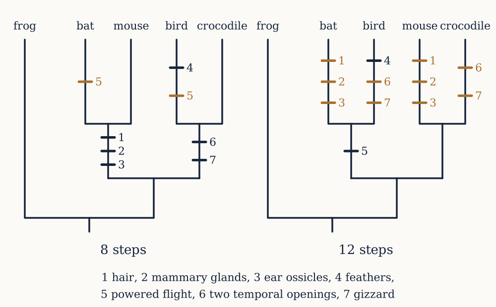
Deep time and extinction

Any explanation of adaptation by small accumulated changes is a promissory note drawn on a bank account nobody had checked, and the previous lesson ended by naming the currency: time.

The account was checked, and by people with no interest in biology. This lesson follows three separate findings, each established before Darwin published and none of them by him: that the earth is very old, that species go extinct, and that the fossils in the rocks appear in a fixed order that is never inverted. It ends with the first serious mechanism proposed for that order, and with the experiment that killed it.

An earth with no visible beginning

In 1788 James Hutton took two companions by boat to Siccar Point on the Berwickshire coast to show them a rock face. At the bottom are beds of greywacke standing almost vertically. Above them, cut flat across their broken ends, lie beds of red sandstone lying nearly horizontally. To read that face you must accept a sequence: the greywacke was laid down flat under water, buried, tilted to the vertical, lifted above sea level, planed off by erosion, submerged again, and buried again under sand. Every one of those steps happens today at rates you can measure, and none of them is quick.

Hutton's argument, later made systematic by Charles Lyell in the Principles of Geology of 1830 to 1833, is that the processes visible now are enough to account for everything visible in the rocks, given enough time. He would not name the time. What he wrote is that the record shows "no vestige of a beginning, no prospect of an end", which is not a measurement but a refusal to accept one that was too small.

The refusal is quantitative in spirit even when the numbers are missing, and it is worth doing the arithmetic he could not.

Example. The Grand Canyon exposes about 1,800 m of flat-lying sedimentary rock. Marine sediments today accumulate at rates in the range 0.02 to 0.1 mm a year. How long does 1,800 m take?

At 0.1 mm a year, 1,800 m is 1.8×106 mm, so the time is 1.8×10⁶/0.1=1.8×107 years, or 18 million years. At 0.05 mm a year it is 36 million years. Either figure is already four orders of magnitude past the six thousand years then commonly assumed, and it takes no account of the gaps, of which the canyon has several: below the flat beds lies a tilted sequence and below that a schist, each demanding its own history of burial, deformation and erosion before the beds above began.

Now you. The chalk of southern England is about 500 m thick and is made almost entirely of the skeletons of single-celled algae, which settle at something like 0.03 mm a year. How long was the chalk sea in place?

Answer

500{,}000/0.03=1.7×107 years, about 17 million. The modern date for the chalk, from the fossils and from radiometric ages in interbedded ash layers, is roughly 100 to 66 million years ago, which is a span of the right order. The point is not the agreement, which is partly luck given the crudity of the rate. The point is that the calculation is the sort a farmer could do, requires no theory, and gives an answer nobody wanted.

Cuvier proves that species end

The second finding came from a man who spent his career arguing against evolution. On 4 April 1796 Georges Cuvier read a paper to the Institut National in Paris comparing the jaws and teeth of living and fossil elephants. He showed that the Indian and African elephants are two distinct species, not varieties of one; that the Siberian mammoth is a third, differing in the shape of the lower jaw and the enamel plates of the molars; and that the great animal from the Ohio, later named mastodon, is a fourth, with blunt conical cusps rather than plates.

The conclusion is the one nobody had been willing to draw. Elephants are not animals that hide. If the mammoth existed and no mammoth is alive, then a species has ended. Within a few years Cuvier had added the giant ground sloth Megatherium, a marine reptile from Maastricht that he identified as a lizard rather than a whale, and a flying reptile he named Ptéro-dactyle. He was the best comparative anatomist alive, his identifications held, and extinction became a fact.

Cuvier's own explanation was a series of geological revolutions, sudden floods that wiped out faunas which were then replaced by immigration from elsewhere. He rejected transmutation flatly and had a good reason for doing so: the mummified ibises brought back from Egypt were three thousand years old and anatomically identical to living ones, so species were evidently stable on any timescale then imaginable. He was right about the observation and wrong about what it implied, because three thousand years is nothing.

The order in the rocks is fixed

The third finding came from a canal surveyor. Between 1799 and 1815 William Smith worked out that strata in England can be identified anywhere by the fossils in them, that the same assemblage always occurs in the same position relative to other assemblages, and that the order never reverses. His 1815 map of England and Wales was drawn on that principle and is still substantially correct.

This is the principle of faunal succession, and its strength is that it is a very easily broken rule. There are thousands of exposures, on every continent, and every one of them is an independent chance to find an assemblage out of place. None does. Trilobites occur below the first fish and never above the last chalk. Flowering plant pollen appears in the Cretaceous and never below it. Mammals with placentas do not occur in Devonian rocks, and no amount of searching has produced them; J. B. S. Haldane, asked what observation would destroy the theory, is supposed to have said a fossil rabbit in the Precambrian.

Note carefully what succession establishes and what it does not. It establishes that different faunas occupied the same place at different times, in a consistent global order. It does not by itself establish that the later ones descended from the earlier ones: Cuvier read the same order as a sequence of replacements. Succession is a constraint that any theory must fit, not a theory.

Kelvin's objection, which was valid

By the 1860s geologists were speaking freely of hundreds of millions of years, and the best physicist in Britain told them they could not have it. William Thomson, later Lord Kelvin, argued in 1862 that the earth began molten and has been cooling by conduction ever since, and that the temperature gradient measured in mines therefore fixes how long the cooling has run. Deep mines gave about 1 °F per 50 ft, which is 36.4 K per kilometre.

Example. Kelvin's conduction model gives the age as t=(Tm/G)2/(πκ), where Tm is the initial surface temperature, G the present gradient and κ the thermal diffusivity of rock. Take Tm=3900 K, G=0.0364 K/m and κ=1.2×10⁻⁶ m² per second. What age comes out?

The length Tm/G=3900/0.0364=1.07×105 m. Squaring gives 1.15×10¹⁰ m², and dividing by πκ=3.77×10⁻⁶ m² per second gives 3.05×10¹⁵ seconds. A year is 3.16×10⁷ seconds, so the age is 9.6×10⁷ years, about 100 million. Kelvin published 98 million with a range of 20 to 400 million, and by 1897 he had narrowed it to between 20 and 40 million. That is not enough time for the geology, let alone the biology, and Darwin called it one of his sorest troubles.

Now you. The calculation is arithmetically correct and its conclusion is wrong by a factor of about a hundred. Where is the error, and what does the episode teach about arguments of this shape?

Answer

Two errors, and the better known is the smaller one. Radioactivity, discovered in 1896, means the earth has a heat source inside it, so the gradient is not the fading trace of an initial store and the clock reads long. The deeper error was identified by John Perry in 1895, before radioactivity was relevant: the model assumes heat moves through the whole earth by conduction, and if the interior convects instead it delivers heat to the base of a cool rigid shell far faster, which reproduces the observed surface gradient at any age you like. Kelvin dismissed him. The lesson is about the shape of the argument: a valid deduction from a measured quantity is only as good as its model of the system, and a physical argument that contradicts a large body of field observation is at least as likely to have a missing term as the field observation is to be wrong.

Putting numbers on it

The resolution arrived with the same discovery that broke the objection. Radioactive decay is a clock: a parent nuclide decays to a daughter at a rate no chemical or physical condition alters, so a mineral that incorporated parent and excluded daughter when it crystallised records its own age in the ratio of the two. Bertram Boltwood applied this to uranium and lead in 1907 and got ages up to 2.2 billion years. Arthur Holmes spent forty years making the method trustworthy. In 1956 Clair Patterson, measuring lead isotopes in the Canyon Diablo iron meteorite, gave the age of the solar system as 4.55 ± 0.07 billion years, a figure that has moved only in its third digit since.

The arithmetic is a rearranged exponential decay. If D is the daughter accumulated and P the parent remaining, then D/P=eλt-1, so t=ln(1+D/P)/λ, with λ=ln2/t1/2.

Example. A zircon crystal contains lead-206 and uranium-238 in the ratio D/P=0.50. The half-life of uranium-238 is 4.468 billion years. How old is the crystal?

The decay constant is λ=0.693/4.468=0.1551 per billion years. Then t=ln(1.50)/0.1551=0.4055/0.1551=2.61 billion years. Zircon is used because it takes uranium into its lattice readily and rejects lead almost completely, so the assumption that all the lead-206 present is decay product is a good one, and because it survives metamorphism that resets other minerals.

Now you. A second zircon from the same terrain gives D/P=0.25. How old is it, and what does the pair of ages mean?

Answer

t=ln(1.25)/0.1551=0.2231/0.1551=1.44 billion years. The pair means the terrain contains crystals that formed more than a billion years apart, which is ordinary: an igneous body can pick up older zircons from the rock it intrudes, and those inherited grains keep their own ages. This is why a single date is nearly worthless and a population of dates is informative. The oldest terrestrial zircons, from the Jack Hills of Western Australia, give about 4.4 billion years.

The first mechanism, and the experiment that killed it

With extinction real, succession established and time eventually granted, the field had a fact needing a mechanism. The first serious one was published by Jean-Baptiste Lamarck in Philosophie Zoologique in 1809, and he deserves better than the caricature.

Lamarck proposed two principles. The first is use and disuse: an organ exercised repeatedly develops and strengthens, one neglected weakens and shrinks. That is simply true, and any bodybuilder demonstrates it. The second is that such acquired modifications are passed to offspring. Together they give a mechanism that is genuinely adaptive, since the changes are directed at what the animal actually does, and Lamarck combined it with a separate drive towards complexity to produce the first full theory of transmutation in print.

The second principle is the one that must be tested, and unlike most nineteenth-century biology it is directly testable. August Weismann did the obvious experiment in the 1880s, cutting the tails off mice and breeding them. The reported result is 901 young over five generations, every one with a normal tail. The experiment is often mocked as naive, since nobody claimed that mutilation is an adaptive response, and the criticism is fair; but the theoretical point that replaced it was Weismann's own and it is decisive. In animals the cells that make gametes are set aside early and are not the cells that build the body. Information flows from germ line to body, and there is no return path, so what the body acquires cannot be written back.

The modern qualifications should be stated honestly, because they are real and are routinely overstated. Chemical marks on DNA and its packaging proteins can persist through cell division, and in plants and a few animal cases can survive into the next generation or two. These effects are found, they are usually reset within a couple of generations, and they do not alter the DNA sequence. They are a mechanism for short-term response, not the mechanism for building an eye. Lamarck's fact, that lineages change over time, survived. His mechanism did not.

That leaves the field where the next lesson begins: an old earth, a documented succession of faunas, a proven history of extinction, and no working account of how one fauna gives rise to the next.

Darwin's argument

The previous lesson left a fact without a mechanism: faunas succeed one another in a fixed order over an enormous span of time, and nothing explains how one gives rise to the next.

Charles Darwin supplied the mechanism, and the striking thing about it is how little it needs. There is no new force, no vital principle, no drive towards complexity. There are four observations, all of them agreed on by his opponents, and the conclusion follows from them by ordinary reasoning. This lesson takes the argument apart, states what it establishes, and is precise about the three things it could not supply in 1859.

The domesticated animals come first

On the Origin of Species was published on 24 November 1859 in a printing of 1,250 copies, and it does not begin with fossils or with the Galapagos. It begins with pigeons.

That is a deliberate choice of ground. Darwin had kept fancy pigeons since 1855 and had joined two London pigeon clubs. The breeds are grotesquely different: the pouter with an inflatable crop and elongated body, the fantail with thirty or forty tail feathers instead of twelve and its head bent back to touch them, the short-faced tumbler with a beak like a finch, the carrier with wattled skin around the eyes and bill. An ornithologist shown their skeletons alone would file them as several genera. Yet every fancier knows they are all Columba livia, the rock dove, because they are interfertile and because crossing two breeds throws back to a slate-blue bird with black wing bars.

Darwin's use of this is precise. Breeders did not design those birds. They selected, generation after generation, from whatever variation turned up, keeping the birds nearest the direction they wanted and killing or selling the rest. Nobody planned the fantail's vertebral count. What the case establishes is that undirected variation plus a sustained bias in who reproduces is sufficient to produce structural change of a magnitude that would be called generic in the wild. The word Darwin uses for the bias is selection, and he took it from the breeders.

The analogy has a well-known weakness, which he states himself: in the domestic case there is a selector with an intention, and in nature there is not. The argument therefore has to supply something that plays the selector's role without wanting anything. That is what Malthus gave him.

Geometric increase against finite resources

Thomas Malthus's Essay on the Principle of Population of 1798 argues that populations increase geometrically while their subsistence increases at best arithmetically, so that population is always pressing against its limit and is always cut back. Darwin read it for amusement in September 1838 and recognised the missing piece at once.

The biological version is stronger than the human one, because reproduction in most species is not close to replacement, it is enormously above it. Darwin makes the point with the slowest breeder he can find.

Example. Darwin's later editions state that from a single pair of elephants, breeding from age 30 to age 90 and producing six young, there would be nearly nineteen million alive after 745 years. What annual rate of increase does that imply, and what is the doubling time?

Starting from 2 and reaching 1.9×10⁷ is a factor of 9.5×10⁶, so e745r=9.5×10⁶ and r=ln(9.5×10⁶)/745=16.07/745=0.0216 per year, about 2.2 per cent. The doubling time is ln2/r=0.693/0.0216=32 years. Two per cent a year is a rate no one would describe as explosive, and it is what the slowest-breeding land animal in the world achieves if nothing kills it. The conclusion Darwin wants follows immediately: since elephants do not cover the earth, almost every elephant born must fail to leave a descendant.

Now you. A bacterium of mass 10-12 g divides every 20 minutes. How long until its descendants weigh as much as the earth, 6.0×1027 g?

Answer

The required increase is 6.0×1027/10-12=6×1039 fold, and the number of doublings is log2(6×1039)=132. At 20 minutes each that is 2,640 minutes, or 44 hours. Under two days. The number is absurd, which is the point: unrestrained geometric increase is not merely fast, it is impossible, so the restraint is universal and continuous. Every population you can see is a population being held down, and the interesting question is which individuals it is held down on.

The argument in four premises

With those two pieces the argument can be stated compactly, and it is worth writing it out because most disputes about it are really disputes about one premise.

First, organisms produce far more offspring than can survive, as the elephant arithmetic shows. Second, individuals within a species vary, in every character anyone bothers to measure, and the variation is not confined to trivia. Third, some of that variation is heritable: offspring resemble their parents more than they resemble the population, which is why breeding works at all. Fourth, some of the heritable variation affects the chance of surviving and reproducing in the circumstances the organism actually faces.

From these four, the conclusion is forced. If more are born than can live, and they differ, and the differences are passed on, and some differences make survival likelier, then the composition of the next generation is not a random sample of the last. The characters that helped are over-represented. Repeat for enough generations and the population is no longer what it was. Darwin called the process natural selection, and later, adopting Herbert Spencer's phrase in the fifth edition of 1869, "survival of the fittest".

Nobody in 1859 denied any of the four premises. What was denied, and reasonably, was that the process could accumulate far enough to build an eye or to split a lineage. Darwin's answer occupies the other thirteen chapters: it consists of showing that the process, if real, would leave a specific set of traces, and then showing that those traces are present. Geographical distribution, the peculiarities of island faunas, rudimentary organs, the classification hierarchy of the previous lesson, and the imperfection of the fossil record are all handled this way. He called the book "one long argument", and it is a fair description of a structure that never has a single decisive experiment in it.

Example. A critic says that selection cannot create anything, since all it does is remove the unfit, and removal is not creation. Which premise is being attacked, and is the objection sound?

None of the four is being attacked, which is the first thing to notice: the objection is aimed at the conclusion by way of a claim about what the word "creation" can mean. It is unsound, and the reason is the third premise. Selection removes individuals, but what persists across generations is not individuals, it is heritable variants, and a variant that was rare can be made common. Combine that with the fact that variation keeps arising in each generation, and a favourable combination that no single ancestor possessed can be assembled step by step, because each step is retained by heredity while the next is being waited for. The process is cumulative, and it is the cumulation, not the removal, that does the building. Darwin's own answer was the breeder's: nobody says a fancier created nothing merely because all they did was choose which birds to keep.

Now you. A second critic accepts all four premises but says the conclusion holds only for small changes within a species, not for the origin of new ones. Is that a coherent position, and what would settle it?

Answer

It is entirely coherent, it was the majority view among naturalists for decades after 1859, and it cannot be refuted from the four premises alone. They license the claim that populations change; they do not by themselves license the claim that the change can accumulate without limit, or that it can produce two lineages incapable of interbreeding. What settles it is evidence of three separate kinds: a demonstration that no internal barrier stops the accumulation, which needs a theory of heredity Darwin did not have; direct observation of reproductive isolation arising, which came later; and the historical record of the intermediates, which is what the fossils and the genomes supply. Three of the remaining lessons in this course exist to answer this objection, and taking it seriously rather than dismissing it is the reason the answer is worth having.

Darwin against himself

Chapter six is titled "Difficulties on Theory", and it contains the strongest statements of the case against that anyone wrote in the century. This is not modesty, it is tactics: an objection you have stated better than your opponent cannot be used against you.

The famous one is the eye. Darwin writes that to suppose the eye, with all its inimitable contrivances, could have been formed by natural selection seems, he freely confesses, absurd in the highest possible degree. Then he answers his own point in two moves. If a graded series of eyes exists, each useful to its possessor, and if the variation is heritable, then the difficulty is only apparent. He goes through the series the invertebrates actually provide: a pigmented spot, a pit, a deeper pit that gives direction, a narrowed aperture that makes a pinhole image, a filled chamber, a lens. Every stage in that list is the working eye of some living animal, which is what makes it an argument rather than a story.

Example. Why is Darwin's move here logically stronger than simply asserting that the eye evolved gradually?

Because it converts a claim about the possible into a claim about the actual. The objection is that intermediate stages of an eye would be useless, so selection could not preserve them. If you can exhibit living animals at each intermediate stage, thriving, the objection's premise is false as a matter of observation and no argument about probability is needed. The structure recurs throughout the book: identify what your opponent claims to be impossible, then find it living somewhere. The limitation is equally clear, and Darwin does not hide it: showing that a series of viable intermediates exists does not show that any actual eye passed through that series, which is a historical claim needing evidence of a different kind.

Now you. Chapter six also raises the problem of sterile worker castes in ants, which leave no offspring at all. Why is this a sharper problem for the argument than the eye, and what does Darwin's answer commit him to?

Answer

The eye is a question of degree, but the workers look like a direct contradiction: a character that reduces its bearer's reproduction to zero cannot be favoured by a process defined in terms of its bearer's reproduction. Darwin calls it the one special difficulty which at first appeared to me insuperable and actually fatal to my whole theory. His answer is that selection can act on the family rather than the individual, since a well-provisioned colony leaves more fertile queens and the queen carries the tendency to produce such workers. That commits him to selection operating on a unit larger than the organism, which is exactly the ground on which the theory would be fought over for another century. The last lesson of this course returns to it with the arithmetic Darwin lacked.

Wallace, and what independent discovery shows

On 18 June 1858 Darwin, who had been accumulating evidence for twenty years without publishing, received a manuscript from Alfred Russel Wallace, then collecting specimens in the Moluccas. It set out selection acting on variation under the pressure of population, from Malthus, and asked Darwin to forward it to Lyell if he thought it worth anything. Darwin wrote that he never saw a more striking coincidence, and that if Wallace had his 1842 sketch he could not have made a better short abstract of it.

The compromise arranged by Lyell and Joseph Hooker was a joint reading at the Linnean Society on 1 July 1858, of Wallace's essay together with extracts from Darwin's unpublished 1844 essay and an 1857 letter. It attracted no attention whatever; the society's president reported at the end of the year that nothing striking had occurred. Darwin then wrote the Origin in thirteen months as an "abstract" of the much larger book he had planned.

The joint discovery is worth a moment. Wallace and Darwin differed in temperament, class, income and continent, and shared two things: field experience of geographical variation, and Malthus. That two people reasoning independently from the same premises reached the same conclusion is weak evidence that the conclusion follows from the premises rather than from the person, which is the most that such coincidences ever show. They later disagreed sharply, Wallace holding that natural selection could not account for the human intellect, so their agreement was not a matter of shared prejudice.

The three things the argument did not have

It is easy to read the Origin as the end of the story. It is better read as an argument with three specified holes, all of which Darwin knew about.

It had no theory of heredity. Darwin needed offspring to resemble parents and could not say why they do. His own attempt, pangenesis, published in 1868, supposed that every part of the body sheds particles called gemmules that collect in the reproductive organs; it is a blending theory, it is Lamarckian in effect since a modified organ would shed modified gemmules, and it is wrong. Worse, blending of any kind is fatal to the argument, for a reason a Scottish engineer would state in 1867 and the next lesson takes up.

It had no account of where variation comes from. Darwin treats variation as a given, uses the phrase "the laws governing inheritance are quite unknown", and is explicit that his ignorance is profound. Since the whole process is a filter, and a filter cannot produce what is not fed into it, this is a gap in the middle of the mechanism and not at its edge.

It had no time, in the sense of the previous lesson: Kelvin's twenty to forty million years was not enough, and Darwin's own estimate of 300 million years for the erosion of the Weald, printed in the first edition, was attacked so effectively that he removed it from later ones.

Two of those three would be filled by the same discovery, made three years after the Origin appeared, in a monastery garden in Brno, and ignored for thirty-four years.

The heredity problem

An engineer reviewing the Origin of Species in 1867 found a hole in it that Darwin could not close, and closing it required knowing something about heredity that nobody in Britain knew.

The previous lesson set out the four premises of the argument and named its weakest joint: Darwin needed offspring to resemble their parents and had no account of why they do. This lesson is about what goes wrong when you assume the obvious account, and about the seven years of pea breeding that gave the right one.

Jenkin's objection

Fleeming Jenkin was a telegraph engineer, a colleague of Kelvin's, and a good enough critic that Darwin said he had given him more trouble than any other reviewer. His review appeared in the North British Review in June 1867 and it makes two arguments.

The first is about the limits of selection. Breeders, Jenkin observed, get rapid change at first and then hit a wall: a racehorse line improves and then stops improving, and no amount of further selection carries it past. If domestic selection has a boundary, why should natural selection not have one too?

The second is the swamping argument, and it is the serious one. Suppose a single individual is born with some markedly favourable variation. It must mate with an ordinary member of the population. If inheritance blends, meaning that the offspring is intermediate between its parents, then its young carry half the novelty, their young a quarter, and the variation is diluted out of existence long before selection has had time to act on it. Jenkin illustrated this with an offensive parable about a shipwrecked European on an island, which is the part everybody remembers and the least important part of the argument.

Darwin's defence was that he did not rely on single sports but on the small continuous variation present everywhere in a population. That is a real answer to the parable, but it does not touch the underlying arithmetic, and the arithmetic is worth doing.

Example. Under strict blending, an offspring's value for some measured character is the average of its two parents' values. If parents pair at random, what happens to the variance of the character in each generation?

Let the character have variance V in the parental generation, and let the two parents of any offspring be drawn independently. The offspring's value is (x1+x2)/2, so its variance is

operatorname{Var}(x1+x22)=V+V4=V2

The variance halves every generation, whatever it started at, and it does so with no selection acting at all. After 5 generations V is down to 3.1 per cent of its original value, after 10 generations to 0.098 per cent, and after 20 to one part in a million. A blending population becomes uniform, and a uniform population cannot be selected on, because every individual is the same.

Now you. To keep the variance steady under blending, how much new variation must be supplied each generation, and what does that requirement imply?

Answer

Exactly half of the standing variance must be created anew every generation, since half is destroyed. R. A. Fisher pressed this in 1930: the required rate of fresh variation is so enormous that it would have to be visible, with something like half the population carrying a newly arisen difference in every character in every generation, which nobody observes. Under particulate inheritance the requirement collapses to almost nothing, because the variance is not destroyed in the first place and mutation has only to replace what selection and chance remove. The blending model is not merely inconvenient for Darwin. It is quantitatively incompatible with populations that are observably variable.

Why peas, and why counting

The answer was already in print. Gregor Mendel, an Augustinian friar at St Thomas's Abbey in Brno, had studied physics and mathematics at Vienna under Christian Doppler between 1851 and 1853, and returned to a monastery with an experimental garden. Between 1856 and 1863 he grew something like 28,000 pea plants, and he read the resulting paper to the Brno Natural History Society on 8 February and 8 March 1865, publishing it in the society's proceedings in 1866.

Almost everything about the design is better than what botanists were doing. The garden pea has many varieties that breed true, so the starting material is clean. Its flower is closed and normally self-pollinates, so a plant left alone is a controlled experiment and a cross has to be made deliberately with forceps. Above all, Mendel chose characters that come in two sharply distinct states with nothing in between: the seed is round or wrinkled, the cotyledons yellow or green, the stem tall or short. There is no judgment involved in scoring them, so a character can be counted rather than described.

Counting is the innovation. Earlier hybridisers, including some very good ones, recorded which forms appeared. Mendel recorded how many, in numbers large enough to have a standard error worth quoting, and he treated one character at a time rather than trying to describe the whole plant at once.

Segregation, and a ratio of three to one

Crossing a true-breeding round-seeded plant with a true-breeding wrinkled-seeded one gives an F1 generation that is entirely round. The wrinkled character has not been blended away to something intermediate, and Mendel's crucial observation is that it has not been destroyed either: self-pollinating the F1 gives an F2 in which wrinkled seeds reappear, unchanged, at about a quarter.

The model that explains this is that each plant carries two copies of a factor for the character, one inherited from each parent; that the copies do not mix; that one form of the factor (round) masks the other (wrinkled) when both are present; and that the two copies separate when gametes are made, so each gamete carries one at random. A cross of two F1 plants, each carrying one of each, then produces the four equally likely combinations, three of which contain at least one round factor.

Example. Mendel counted 5,474 round and 1,850 wrinkled seeds in the F2. Test this against the 3:1 prediction.

The total is 5474+1850=7324, so the expected counts are 0.75×7324=5493.0 round and 0.25×7324=1831.0 wrinkled. The chi-square statistic is

χ2=(5474-5493)25493+(1850-1831)21831=0.066+0.197=0.263

On one degree of freedom that has a probability of about 0.61, meaning a random sample would deviate from 3:1 by more than this in about three cases out of five. The observed ratio is 2.96 to 1. Pooling all seven characters gives 14,949 dominant to 5,010 recessive, a ratio of 2.984, on nearly 20,000 seeds.

Now you. Why is it essential to the argument that the wrinkled seeds in the F2 are indistinguishable from the original wrinkled parent, rather than merely wrinkled-ish?

Answer

Because that is the whole difference between particulate and blending inheritance. Under blending, a character that vanishes in the F1 is gone: there is nothing left to reappear. Mendel's wrinkled seeds come back at full strength after a generation of complete concealment, which shows that the factor passed through the F1 plant unaltered by the round factor it shared a cell with. Heredity is therefore the transmission of discrete objects, not the mixing of fluids, and the variance-halving arithmetic of the previous section simply does not apply. Everything Darwin needed follows from this one observation.

Two characters at once

Mendel then crossed plants differing in two characters at once, round yellow against wrinkled green, and asked whether the two behave independently. If they do, the F2 should show the product of two independent 3:1 ratios, which is 9:3:3:1.

Example. Mendel's dihybrid F2 gave 315 round yellow, 108 round green, 101 wrinkled yellow and 32 wrinkled green. Does that fit 9:3:3:1?

The total is 556, so the expected counts are 556×9/16=312.75, 556×3/16=104.25 twice, and 556×1/16=34.75. Then

χ2=2.252312.75+3.752104.25+3.252104.25+2.75234.75=0.016+0.135+0.101+0.218=0.470

On three degrees of freedom that has a probability of about 0.93. The fit is excellent, and two of the four F2 classes, wrinkled yellow and round green, are combinations that did not exist in either grandparent. Independent assortment does not merely preserve variation; it manufactures new combinations of it, which is a second thing Darwin needed and could not supply.

Now you. Independent assortment is not a general law. What breaks it, and does the breach damage the argument above?

Answer

Genes sitting close together on the same chromosome are inherited together and do not assort independently. William Bateson and Reginald Punnett found ratios badly departing from 9:3:3:1 in sweet peas around 1905 and could not explain them; Thomas Hunt Morgan's group explained them from 1911 as linkage, with the frequency of recombination between two loci measuring the distance between them. Mendel's seven characters actually map to only four of the pea's seven chromosome pairs, so some of his pairs were on the same chromosome and happened to be far enough apart to assort nearly freely. The breach does not damage the argument. Linkage reduces the rate at which new combinations are produced without abolishing it, because crossing over reshuffles even linked loci, and the essential point, that factors are discrete and are not diluted, is untouched.

The data are too good

There is an awkwardness about Mendel's numbers that an honest account has to include. In 1936 R. A. Fisher, who admired the work and reconstructed the whole experimental programme, showed that the agreement between Mendel's observed counts and his expected ratios is closer than sampling would ordinarily produce. Combining the chi-squares across all the experiments Fisher obtained a total of about 41.6 on 84 degrees of freedom, where the expected value of a chi-square is its degrees of freedom. Deviations that small arise by chance far less than one time in ten thousand.

Fisher also identified a specific technical problem. To distinguish a true-breeding round F2 plant from a segregating one, Mendel raised its offspring and looked for any wrinkled seed. With ten seeds scored, a segregating plant has a probability (3/4)10=0.056 of producing no wrinkled seed at all and being misclassified. That shifts the expected ratio of segregating to constant plants from 2:1 down to about 1.70:1. Mendel reported 372 segregating to 193 constant, a ratio of 1.93, which sits close to the naive expectation and away from the correct one.

What to conclude is disputed and the honest answer is that we do not know. Proposals include unconscious bias in scoring ambiguous seeds, a gardening assistant who knew what was wanted, stopping data collection when the ratio looked right, and Fisher having mismodelled the number of seeds actually scored. Nobody has suggested the conclusions are wrong: the ratios have been reproduced thousands of times since, in peas and in everything else. The episode is a good illustration of the difference between a result being true and a data set being trustworthy, and of the fact that the two can be separated by experiment.

Rediscovery, and a thirty-year war

Mendel's paper was distributed to about 130 institutions and cited a handful of times before 1900, when three botanists, Hugo de Vries, Carl Correns and Erich von Tschermak, published segregation ratios independently and found the paper in the literature. William Bateson read it on a train to London, abandoned his lecture notes, and became its advocate in Britain.

The expected outcome would have been the immediate union of Mendel with Darwin. What happened instead was twenty-five years of hostility. The Mendelians, led by Bateson and by de Vries, studied characters with two sharply distinct states and concluded that evolution proceeds by discrete jumps: de Vries's mutation theory, based on abrupt new forms appearing in the evening primrose, held that new species arise in a single step and that selection merely weeds out the failures. The biometricians, led by Karl Pearson and W. F. R. Weldon, studied characters like height, weight and beak size, which vary continuously with no distinct classes at all, had built statistics in order to measure the resemblance between relatives, and pointed out that these characters are the ones selection actually works on in nature.

Each camp was right about its own data and wrong about the other's, and the dispute was bitter enough to be personal. It looked like a real contradiction: if heredity comes in discrete units producing sharp ratios, where does smooth continuous variation come from, and how can selection move a population by small degrees if the underlying units come only in whole numbers?

The resolution is arithmetical rather than experimental, and it needs a shift of attention from the family to the population. That shift, made in a single page of Science in 1908, is the subject of the next lesson.

Populations and frequencies

A question asked from the floor of a scientific meeting in 1908 exposed the fact that nobody yet knew what Mendel's rules imply about a whole population, as opposed to a single family.

The previous lesson ended with two camps convinced they had incompatible sciences: discrete factors giving sharp ratios on one side, smooth continuous variation and the resemblance of relatives on the other. Both were right. Reconciling them requires changing the object of study from the pedigree to the population, and once that change is made the theory acquires something it had lacked since 1859: a number to measure.

Yule's question

At a meeting of the Royal Society of Medicine, Reginald Punnett presented Mendelism, and G. Udny Yule asked an awkward question. Brachydactyly, a condition producing short fingers, is inherited as a dominant. If dominants are three times as common as recessives in an F2, should not brachydactyly gradually rise until three-quarters of the population has short fingers? It plainly has not. Does that not tell against the whole scheme?

Punnett could not answer on the spot, and took the question to his cricketing acquaintance G. H. Hardy, a Cambridge pure mathematician who regarded the problem as trivial and the fuss as evidence that biologists could not do algebra. Hardy's reply appeared as a short letter in Science on 10 July 1908 under the title "Mendelian proportions in a mixed population". Wilhelm Weinberg, a physician in Stuttgart, had published the same result six months earlier in German, and the result carries both names.

Yule's error is a good one to have made, because it is the natural reading. The 3:1 ratio is a statement about the offspring of a particular cross, two heterozygotes, and says nothing about how common that cross is. To answer the question you have to ask what fraction of the population carries each allele, which is a quantity nobody had thought to define.

The result

Consider one locus with two alleles, A and a. Let p be the fraction of all the gene copies in the population that are A, and q=1-p the fraction that are a. Assume mating is at random with respect to this locus, that the population is large enough for sampling error to be negligible, and that nothing kills, mutates or immigrates differentially.

Under random mating, a zygote is formed by drawing two gametes independently from the pool. The chance of drawing A twice is p2, the chance of a twice is q2, and the chance of one of each is 2pq, the factor of two counting the two orders. So the genotype frequencies are

AA:Aa:aa=p2:2pq:q2

The second half of the result is the important half. Work out the allele frequency in this new generation. Every AA contributes two A copies and every Aa contributes one, so

p=2p2+2pq2(p2+2pq+q2)=p2+pq1=p(p+q)=p

The frequency is unchanged. It will be unchanged next generation and the one after. Nothing happens.

That is the answer to Yule. Dominance describes how an allele is expressed when paired with another, not how often it occurs, and expression has no bearing on transmission. A dominant allele at 1 per cent stays at 1 per cent forever unless something acts on it, and a recessive at 99 per cent stays there.

Why a null model is worth having

It is easy to dismiss the Hardy-Weinberg result as an accounting identity, and in one sense it is. Its value is that it is the first statement in biology of what happens when nothing happens, and every science needs one of those. Newton's first law is not interesting because objects often move at constant velocity; it is interesting because it identifies which observations require a force.

The list of assumptions is therefore not a weakness but the actual content. Genotype frequencies depart from p2:2pq:q2, or allele frequencies move between generations, only if at least one of the following fails: random mating, a population large enough to ignore sampling, no selection on the locus, no mutation at the locus, no migration in or out, and equal frequencies in the two sexes at an autosomal locus. Each failure is a named evolutionary force, and the remaining lessons of the first half of this course take them one at a time.

The result also supplies a definition. Evolution is a change in allele frequency in a population across generations. That is deliberately narrow and it is what makes the subject quantitative. It says nothing about progress, complexity or species, and it locates evolution in a population rather than in an individual, which is why the statement that an individual organism does not evolve is not a pedantic quibble but a consequence of the definition.

Example. Cystic fibrosis is recessive and affects about one in 2,500 births in northern European populations. What fraction of that population carries one copy?

Affected individuals are the aa class, so q2=1/2500=0.0004 and q=0.02. Then p=0.98, and the carrier frequency is

2pq=2×0.98×0.02=0.0392

about 3.9 per cent, or one person in 26. Note the ratio of carriers to affected individuals, 2p/q=2×0.98/0.02=98. For every child with the disease there are 98 unaffected carriers, so almost all copies of the allele are in people who will never show it. That fact governs how quickly selection can remove a rare recessive, and the next lesson makes it quantitative.

Now you. Phenylketonuria affects about one in 10,000 births in the same populations. What is the carrier frequency, and how many carriers are there per affected person?

Answer

q2=10-4, so q=0.01 and p=0.99. Carriers are 2pq=2×0.99×0.01=0.0198, about 2 per cent, or one person in 51. The ratio of carriers to affected is 2p/q=1.98/0.01=198. Making the disease ten times rarer does not make the allele ten times rarer, only about three times, because the affected frequency goes as the square of the allele frequency. This square is the single most useful thing about the Hardy-Weinberg result in practice: it converts a countable clinical incidence into an allele frequency you could not otherwise observe.

Testing a population against the null

Because it predicts genotype frequencies from allele frequencies, the result is testable on any sample where genotypes can be scored directly.

Example. A survey types 1,000 people at a locus with two codominant alleles, so all three genotypes can be distinguished, and finds 298 MM, 489 MN and 213 NN. Does the sample fit Hardy-Weinberg proportions?

First get the allele frequency by counting copies. There are 2×298+489=1085 copies of M out of 2000, so p=0.5425 and q=0.4575. The expected counts are then p2N=294.3, 2pqN=496.4 and q2N=209.3, and

χ2=3.72294.3+7.42496.4+3.72209.3=0.047+0.110+0.065=0.22

On one degree of freedom, since the allele frequency was estimated from the same data, that is a very good fit. Human blood group loci generally do fit this well, which is worth knowing: it means that for most loci, most of the time, none of the forces is acting strongly enough to see in a sample of a thousand.

Now you. A different sample of 1,000 gives 357, 485 and 158. Compute the fit, and say what a large excess of homozygotes would have indicated had one appeared.

Answer

Copies of the first allele number 2×357+485=1199, so p=0.5995, q=0.4005, and the expected counts are 359.4, 480.2 and 160.4. Then χ2=0.016+0.048+0.036=0.10, again a good fit. An excess of homozygotes in both directions, with a deficit of heterozygotes, has three standard causes and they are hard to tell apart from one sample: inbreeding, which pairs relatives and therefore pairs identical alleles; the Wahlund effect, where the sample unknowingly pools two populations with different allele frequencies; and a null allele that fails to amplify in the assay, so that heterozygotes are misread as homozygotes. The third is a laboratory artefact and is the commonest explanation in practice, which is a useful corrective to reading every departure as biology.

Where continuous variation comes from

The Hardy-Weinberg result settles Yule's question, but the deeper quarrel of the previous lesson was about continuous characters. Human height has no classes: it is a smooth distribution with no gaps, and no amount of pea breeding produces anything like it. How can discrete factors give that?

The answer, suggested by Yule himself in 1902 and worked out completely by R. A. Fisher in 1918, is that they give it as soon as more than one locus affects the same character. Suppose a character is influenced by n loci, at each of which one allele adds a unit to the measurement and the other adds nothing, and that the alleles are at frequency one half. An individual carries 2n alleles, of which some number are the adding kind, so the character takes one of 2n+1 values with binomial frequencies.

Example. Take one locus, then two, then six. How many phenotypic classes are there, in what proportions, and how common is the most extreme individual?

With one locus there are three classes in the proportions 1:2:1, and the extreme occurs at frequency 1/4. With two loci there are five classes, 1:4:6:4:1, and the extreme is 1/16. With six loci there are thirteen classes, 1:12:66:220:495:792:924:792:495:220:66:12:1, and the extreme is 1/4096. Thirteen classes spread over a range of twelve units, with a standard deviation of 12×0.25=1.73 units, is already a bell-shaped distribution in which neighbouring classes differ by less than the measurement error of most instruments. Add any environmental contribution and the classes smear into each other completely.

Now you. Two tall parents of the same height sometimes produce a child taller than either. Blending inheritance cannot allow this. Why does the multiple-factor model allow it easily?

Answer

Because the parents' identical measurements can rest on different combinations of alleles. If height is set by six loci and each parent carries seven adding alleles out of twelve, they look the same, but one may carry them at loci 1 to 4 and the other at loci 3 to 6. Their child draws one allele from each parent at each locus and can easily assemble eight or nine adding alleles, exceeding both parents. This is transgressive segregation, it is routine in plant and animal breeding, and it is a direct prediction of particulate inheritance that blending forbids. It is also the reason selection can push a population beyond the range of any individual it started with, which is precisely what Fleeming Jenkin said could not happen.

What is now available and what is missing

The two camps were arguing about nothing. Continuous characters are Mendelian characters counted several at a time, the resemblance between relatives that the biometricians measured is exactly what the multiple-factor model predicts, and Fisher's 1918 paper derived the correlations between parents, siblings and cousins from Mendelian assumptions and matched them to Pearson's own data. The synthesis that name-checks Fisher, J. B. S. Haldane and Sewall Wright is built on this reconciliation, and the field it created is population genetics.

What the reconciliation delivers to Darwin's argument is the missing premise. Heredity is particulate, so variation is not destroyed by transmission; it is conserved exactly, under the stated assumptions, forever. Selection therefore has a permanent supply to work on rather than a fading one, and the swamping objection is dead.

What it does not deliver is any movement at all. Hardy-Weinberg is a statement that populations sit still. To make anything happen, one of its assumptions has to be broken deliberately, and the first and most important of the breakages is the subject of the next lesson.

How fast selection works

Once evolution is defined as a change in allele frequency, the question of whether selection is strong enough to matter stops being a matter of opinion and becomes a calculation.

The previous lesson established that a population left alone does nothing: allele frequencies sit where they are, generation after generation, and the assumptions behind that result are a list of the ways a population can be made to move. This lesson breaks the first of them, the assumption that every genotype survives and reproduces equally well, and works out how fast the frequency changes when it does.

Fitness is a ratio, not a virtue

The word fitness carries two centuries of unhelpful baggage, so it is worth stating flatly what it means in the algebra. The absolute fitness of a genotype is the average number of offspring an individual of that genotype leaves. Only ratios matter for the frequency of an allele, so the convention is to divide through by the largest, giving a relative fitness w with a maximum of one, and to write the shortfall of any other genotype as a selection coefficient s=1-w.

Three things follow at once. Fitness is a property of a genotype in a particular environment, not of an organism, and certainly not of a species: the same allele can have w=1 in one valley and w=0.6 in the next. It is an average over individuals, so a genotype with high fitness contains individuals who leave nothing. And it counts descendants, not strength, health or longevity, which is why a peacock's tail can raise fitness while lowering nearly everything else about its bearer's condition.

It also has nothing to do with dominance. The previous lesson's answer to Yule was that a dominant allele does not spread because it is dominant, and the same holds here: dominance changes how selection sees a genotype, not how strongly it acts.

The recursion, and what it says about speed

Take one locus with alleles A and a at frequencies p and q. Assign relative fitnesses wAA, wAa and waa. Random mating produces zygotes in Hardy-Weinberg proportions, selection then multiplies each class by its fitness, and renormalising by the mean fitness

w=p2wAA+2pqwAa+q2waa

gives the frequencies among the survivors. Counting allele copies among those survivors gives the frequency in the next generation,

p=p2wAA+pqwAaw

That single line is the whole of one-locus selection theory. Everything below is a special case of it.

The simplest case is the clearest. Suppose the organism is haploid, or equivalently that the heterozygote sits exactly halfway between the homozygotes, and let the favoured type have fitness 1+s against the other's 1. Then the ratio p/q is multiplied by exactly 1+s every generation, so ln(p/q) increases by ln(1+s) per generation and the frequency traces a logistic curve. That is a useful thing to know, because the odds ratio is a straight line in time even though the frequency is not.

Example. An allele with a 1 per cent advantage starts at a frequency of 1 per cent. How many generations until it reaches 99 per cent, and how does that change if the advantage is 10 per cent?

The odds go from 0.01/0.99 to 0.99/0.01, a factor of (99)2=9801. The number of generations is ln(9801)/ln(1.01)=9.190/0.00995=924. With s=0.1 the denominator is ln(1.1)=0.0953 and the answer is 97 generations. A 1 per cent advantage is far too small to detect in any field study anyone could run, and it sweeps an allele through a population in under a thousand generations, which for an annual plant is under a thousand years and geologically instantaneous. This is the single most important number in the subject: selection so weak that it is invisible is still overwhelmingly fast on the timescale the previous lessons established.

Now you. The same allele, again at 1 per cent with a 1 per cent advantage. How long does it take to get from 1 per cent to 2 per cent, and from 50 per cent to 51 per cent? Why are the answers so different?

Answer

From 1 to 2 per cent the odds go from 0.010101 to 0.020408, a factor of 2.02, so the time is ln(2.02)/ln(1.01)=0.703/0.00995=71 generations. From 50 to 51 per cent the odds go from 1 to 1.0408, a factor of 1.0408, and the time is 0.0400/0.00995=4 generations. Selection is roughly eighteen times faster in the middle than at the bottom, because what selection acts on is the difference between the two types weighted by how often they meet the environment, and pq is largest at one half. The two tails are where alleles spend nearly all of their time, which is why a sweep looks like nothing at all for a long while and then happens suddenly.

Melanism, costed

The peppered moth, Biston betularia, is normally pale and speckled, and rests on lichen-covered bark where it is very hard to see. A black form named carbonaria was first recorded near Manchester in 1848. By the end of the century it made up something like 98 per cent of the moths caught in the industrial districts, while remaining rare in rural Dorset and Cornwall. The black form is produced by a dominant allele, so a heterozygote is black.

J. B. S. Haldane used this case in 1924 as the first calculation of a selection coefficient from field data, and it is worth repeating because his conclusion is checkable.

Example. Take the melanic phenotype at 0.1 per cent in 1848 and 99 per cent in 1898, with one generation a year. The melanic allele is dominant. What relative fitness does the pale form need?

Because melanism is dominant, a melanic phenotype frequency of 0.001 means q2=0.999, so q=0.9995 and the allele frequency p is 0.0005. Give the melanic genotypes fitness 1 and the pale homozygote 1-s, so that w=1-sq2 and p=p/w. Iterating that recursion for 50 generations and solving for the s that lands the melanic phenotype on 0.99 gives s=0.333. The pale form is two-thirds as fit as the black, or equivalently the black form is 1/0.667=1.5 times as fit. Haldane's published figure was 50 per cent, and the point he drew from it is the one that mattered in 1924: a selective advantage large enough to do this is small enough that no naturalist watching a wood would ever notice it.

Now you. The Clean Air Act of 1956 reversed the conditions. Around Manchester the melanic form fell from roughly 90 per cent in 1960 to roughly 10 per cent by 1995, again about one generation a year. What is the selection coefficient now acting against melanics, and why is it smaller than the one that put them there?

Answer

Now the melanic genotypes carry the cost. With w=(1-s)(1-q2)+q2 and p=p(1-s)/w, starting from p=0.684 (the value giving 90 per cent melanic phenotypes) and requiring 10 per cent melanic phenotypes after 35 generations, the answer is s=0.15. Published estimates from mark-release-recapture and from the frequency series itself sit between 0.1 and 0.2, so the arithmetic and the fieldwork agree.

It is smaller for a structural reason worth keeping. Selection against a dominant allele is efficient, because every copy of it is exposed in a black moth, so a moderate coefficient moves the frequency quickly. Selection against a recessive, which is what the pale allele suffered on the way up, is inefficient once the recessive is rare, because most copies are hidden in heterozygotes. Getting the melanic allele from 0.0005 to near fixation therefore required a much larger coefficient than removing it does. The asymmetry is not biology, it is arithmetic.

The case has been attacked, and the attacks are worth knowing. Bernard Kettlewell's 1950s experiments, which released marked moths and recovered them, used higher densities than occur naturally and sometimes placed moths on tree trunks in daylight, whereas the moths in fact rest mostly on the undersides of branches. Michael Majerus ran a seven-year experiment answering those criticisms, published after his death in 2012: 4,864 moths released on natural resting positions, with predation scored directly, giving a survival advantage to the pale form of about 9 per cent per day in an unpolluted wood. The mechanism is bird predation, the coefficient is real, and the older experiments were sloppy rather than wrong.

Dominance decides what selection can see

The asymmetry in the moth case is general, and it has a consequence that matters far beyond moths.

Example. A recessive allele is lethal in homozygotes, so waa=0 and everything else is 1. Starting from q=0.01, how many generations of complete lethality are needed to halve the frequency?

For a lethal recessive the recursion simplifies to q=q/(1+q), which rearranges to 1/q=1/q+1: the reciprocal of the frequency rises by exactly one per generation. Halving q from 0.01 to 0.005 means taking 1/q from 100 to 200, which takes 100 generations. Killing every homozygote, in every generation, for a century of human generations, removes half the allele. The reason is in the previous lesson's arithmetic: at q=0.01 the ratio of heterozygous carriers to affected individuals is 2p/q=198, so more than 99 per cent of the copies are in people selection cannot touch.

Now you. What does this imply about proposals to eliminate a recessive disease allele by preventing affected people from reproducing?

Answer

It implies they cannot work, and the numbers were available to the people who proposed them. The eugenic sterilisation laws passed in the United States from 1907 and in several European countries after were justified partly by the claim that heritable defects could be bred out of a population. For a rare recessive, sterilising every affected individual is exactly the lethal-recessive model above, and it takes 100 generations, roughly 2,500 years, to halve an allele already at 1 per cent, while mutation replaces some of what is removed. R. A. Fisher and Lancelot Hogben both made versions of this argument in the 1930s. The policies were unjust on grounds that have nothing to do with algebra, and they were also, on their own stated terms, arithmetically futile.

When selection keeps variation instead of spending it

Every case so far ends with one allele at fixation and the variation gone. Selection is normally a consumer of variation, and that is a problem for a theory that needs variation to keep working. There is one important configuration where it is not.

If the heterozygote is fitter than both homozygotes, neither allele can be eliminated, because whichever becomes rare finds itself mostly in heterozygotes and therefore mostly in the fittest class. Writing wAA=1-s, wAa=1 and waa=1-t, the frequency settles at

q*=ss+t

The sickle-cell polymorphism is the textbook case because all three fitnesses can be estimated. The β-globin allele HbS differs from the normal allele by one base, changing glutamic acid to valine at the sixth position of the beta chain. Homozygotes have sickle-cell anaemia. Heterozygotes are largely healthy and, as A. C. Allison established in 1954 by comparing malarial lowlands with highlands in East Africa, are strongly protected against falciparum malaria; case-control work in Kenya published in 2005 puts the protection against severe malaria at roughly tenfold.

Using the conventional estimates wAA=0.89, wAS=1 and wSS=0.20, the coefficients are s=0.11 against the normal homozygote and t=0.80 against the sickle homozygote, so

q*=0.110.11+0.80=0.121

At that frequency 1.5 per cent of births are SS and about 21 per cent of the population carries the trait, which is close to what is measured across the malarial belt of West and Central Africa. Note the price. The mean fitness at equilibrium is w=0.903, so the population pays a permanent 9.7 per cent reduction in mean fitness to hold the polymorphism. Selection is not an optimiser: it is a bookkeeper that stops where the ledger balances, and here it balances at a point that kills a percentage of every generation's children.

What the algebra assumes, and what it cannot do

The recursion assumes one locus, constant fitnesses, an infinite population and random mating. Real fitnesses vary between years, sites and densities, most characters involve many loci, and populations are finite. Later lessons take those apart. Even so, the one-locus model gets the industrial melanism coefficient right to within the spread of the field estimates, which is the sort of agreement a simple model earns.

The deeper limitation is structural rather than numerical, and it is where this lesson hands over. The recursion moves frequencies. It has no term that makes a new allele. Feed it a population with one allele at a locus and it will return that population unchanged forever, however strong the selection, because p=1 gives p=1. Selection is a filter, and a filter is empty until something is poured into it. Where the alleles come from in the first place is the subject of the next lesson.

Where variation comes from

A filter cannot produce what is not poured into it, and the previous lesson's algebra has no term anywhere in it that makes a new allele.

That is the gap Darwin admitted in the Origin when he wrote that the laws governing inheritance are quite unknown, and it is the last hole in the mechanism. This lesson fills it with three processes that can be measured rather than assumed: mutation, which makes new alleles from copying error; duplication, which makes new genes from whole copies; and recombination, which makes new combinations from old alleles. It also settles the question that decides whether the process is Darwinian at all, which is whether a mutation appears because it is needed.

Counting mutations directly

Until sequencing was cheap, mutation rates were inferred indirectly, from the frequency of a visible disease or from mutant colonies on a plate. Both estimates are contaminated by selection. The clean measurement is to sequence a mother, a father and their child, and count the bases in the child that are in neither parent.

In 2012 Kári Stefánsson's group at deCODE did this for 78 Icelandic families and found about 63 new single-base mutations per child. Dividing by the number of bases the method could reliably call in both copies of the genome, roughly 2.6×10⁹ per haploid set counted twice,

μ=632×2.6×109=1.2×10⁻⁸

per base per generation. The study also found something that indirect methods could never have shown: about 87 per cent of the new mutations came from the father, and the paternal number rose by roughly two mutations for every year of the father's age. That asymmetry has a mechanical cause. An egg is produced after about 23 rounds of cell division and then waits; sperm are produced continuously, through hundreds of divisions by middle age, and each division is a chance to copy a base wrongly.

Example. Of the 63 new mutations in a child, how many land in protein-coding sequence, and what does the answer say about how much of a genome selection can be watching?

Protein-coding exons are about 1.5 per cent of the human genome, so the expected number is 63×0.015=0.94, call it one. Roughly a quarter of random changes in coding sequence are synonymous and change no amino acid, so about 0.7 of a mutation per child alters a protein. That is the entire raw material, per person, on which selection for a better protein can possibly act. The other 62 mutations fall in sequence where most changes have no measurable consequence, which is a fact the neutral theory of a later lesson is built on. Note also what the number rules out: an organism cannot be carrying a large hidden reserve of new coding variants each generation, so evolution has to work with very small per-generation increments, exactly as the previous lesson's selection coefficients require.

Now you. Escherichia coli has a genome of 4.6×10⁶ bases and a per-base mutation rate measured by mutation-accumulation experiments at 2.1×10⁻¹⁰ per generation. How often does a cell acquire a mutation, and how many times is a given base mutated in a single overnight culture of 5×10⁹ cells?

Answer

Per genome per generation the rate is 2.1×10-10×4.6×106=9.7×10⁻⁴, so about one cell in a thousand acquires a new mutation each division. That sounds negligible until the second calculation. In a culture of 5×10⁹ cells, the expected number of cells carrying a mutation at any one nominated base is 5×109×2.1×10-10=1.05, and for one specific substitution at that base it is 0.35.

In other words, a tube of broth left overnight on a bench contains a cell mutated at essentially every position in the genome. The bacterium's low per-base rate and its enormous population size cancel almost exactly, and the practical consequence is that for a bacterial infection the relevant question is never whether a resistance mutation will arise. It is already there before the drug is given.

Do mutations arise in response to need?

That last remark conceals the deepest question in the subject. If bacteria become resistant when exposed to a drug, two accounts fit the observation. Either resistant cells are produced at random beforehand and the drug merely selects them, which is Darwinian, or the drug induces the change in the cells that meet it, which is Lamarckian. Until 1943 nobody had a way to decide, and serious microbiologists held the second view.

Salvador Luria found the test while watching a slot machine at a faculty dance in Bloomington, and worked out the statistics with Max Delbrück. The design is elegant because it does not require you to see a mutation at all, only to count survivors.

Grow many small independent cultures of E. coli from tiny inocula. Also grow one large culture and divide it at the end into samples of the same size. Then plate everything on agar covered with bacteriophage T1, which kills every sensitive cell, and count the resistant colonies.

Example. What does each hypothesis predict for the distribution of colony counts across the independent cultures?

Under the induced hypothesis, resistance is conferred at the moment of contact with the phage, with some small probability per cell. Each plate is then a large number of independent trials with a small success probability, so counts follow a Poisson distribution and the variance equals the mean. That prediction holds whatever the probability is, so it needs no fitted parameter.

Under the mutation hypothesis, resistance arises at random during the growth of the culture, before any phage is present. A mutation in the last division before plating contributes one resistant cell. A mutation twenty divisions earlier contributes a clone of about a million. So the count depends on when the first mutation happened, which varies wildly from culture to culture, and the distribution has a long tail of jackpots and a variance far exceeding its mean. The two hypotheses differ not in the average but in the scatter, which is why the experiment is called a fluctuation test.

Now you. In their experiment 23, twenty independent cultures gave a mean of 11.35 resistant colonies with a variance of about 694, while ten samples drawn from one bulk culture gave a mean of 16.7 with a variance of about 15. Which hypothesis survives, and why is the second set of numbers essential to the argument?

Answer

The independent cultures give a variance-to-mean ratio of 694/11.35=61, sixty times what Poisson allows, with several cultures at zero and at least one over a hundred. The induced hypothesis is dead. The mutation hypothesis is exactly what a jackpot distribution looks like.

The bulk-culture samples are the control, and without them the result proves nothing. If resistant cells are simply hard to count, or clump, or the plating is erratic, every set of counts would be overdispersed and the first result would be an artefact of technique. Samples drawn from one culture share their entire mutational history, so the only remaining variation is sampling and plating error, and they give a ratio of 15/16.7=0.90, essentially Poisson. Technique is clean; the excess variance in the first set is biology.

The cleanest demonstration came later. In 1952 Joshua and Esther Lederberg pressed a velvet pad onto a plate grown without phage and transferred the colony pattern to selective plates, showing that resistant colonies appear at the same positions on replicas, so the resistant cells could be traced back to a plate that had never met the selective agent at all.

Mutation on its own is a feeble force

Mutation supplies alleles, but it is a very weak director of frequencies, and it is worth seeing how weak. If A mutates to a at rate u per generation and nothing else acts, then q increases by u(1-q) per generation, so qt=1-e-ut.

With u=10-8, reaching a frequency of one half takes ln2/u=6.9×107 generations, and after a million generations the allele is still at 1 per cent. Against selection coefficients of the order of 0.01, which the previous lesson showed sweep an allele in under a thousand generations, mutation pressure is negligible as a force. Its role is entirely as a source: it decides what is available, not what happens next. The one place the rate does matter directly is in balancing selection against a deleterious recessive, where the equilibrium frequency q=u/s is set by the rate, which is why rare recessive diseases persist at the frequencies they do.

Duplication, and where a genuinely new gene comes from

Point mutation modifies an existing gene. It does not obviously explain how a genome comes to have more genes than it had, and the objection that selection can only tinker with what exists has real force against point mutation alone.

The answer, argued by Susumu Ohno in 1970, is duplication. Unequal crossing over, retrotransposition and whole-genome duplication all produce a second copy of a gene, and a second copy is free in a way the first is not: while the original continues doing the job, the spare can accumulate changes that would otherwise be lethal. Most spares simply decay into pseudogenes, and the genome is full of those. Occasionally one acquires a function the original did not have.

The cases are specific enough to check. Old World primates see in three colours because an ancestral long-wavelength opsin gene duplicated on the X chromosome and the two copies diverged by a handful of amino acid substitutions, shifting one peak from 560 to 530 nanometres; New World monkeys mostly retain the single gene. Antarctic notothenioid fish survive at temperatures below the freezing point of their blood using an antifreeze glycoprotein whose gene is a modified copy of a trypsinogen, still carrying recognisable fragments of the digestive enzyme's sequence at both ends. The vertebrate globins, myoglobin and the alpha and beta chains of haemoglobin, are one ancestral gene copied and recopied, which is why the beta cluster on human chromosome 11 has five working genes and a pseudogene lying in the order they are used through development.

Rates can be estimated. Michael Lynch and John Conery's 2000 survey put gene duplication at roughly 0.01 per gene per million years, which for a genome of 20,000 genes is about 200 duplications per million years, most of them doomed.

Recombination shuffles what mutation makes

The third source manufactures nothing new at the level of the allele but a great deal at the level of the combination. A human produces gametes by choosing one of each of 23 chromosome pairs independently, which alone gives 223=8.4×10⁶ distinct combinations, and crossing over then breaks and rejoins the chromosomes at one to three points each, so the number of distinguishable gametes is effectively unbounded.

This matters for a reason the previous lessons set up. Selection acting on a population without recombination has to wait for two beneficial mutations to occur in the same lineage, one after the other. With recombination they can arise in different individuals and be brought together, which is Fisher and Hermann Muller's argument for why sex exists at all. Recombination is also what makes the multiple-factor model of the fifth lesson generate transgressive offspring: the child assembling more adding alleles than either parent has is a recombination product.

The arithmetic of supply

Put the rate and the population size together and the picture changes character.

Example. There are about 8×10⁹ people alive. Each carries roughly 63 mutations absent from their parents. How many times over has every base in the human genome been mutated afresh in the living population?

The total is 8×109×63=5.0×10¹¹ new mutations, spread over 3.1×10⁹ sites, which is 163 new mutations per site. Every single position in the human genome exists in a mutated form in someone alive today, roughly a hundred and sixty times over, and every possible single-base variant compatible with reaching birth is currently present somewhere in the species. The limiting resource in human evolution is emphatically not the supply of point mutations.

Now you. Tuberculosis is treated with three or four drugs at once, never one. Resistance to rifampicin arises by point mutation at about 10-8 per cell per generation and to isoniazid at about 10-6. An untreated lung cavity can hold 108 bacilli. Explain the treatment regime in numbers.

Answer

With 108 bacilli, the expected number already resistant to rifampicin is 108×10-8=1, and to isoniazid 108×10-6=100. Single-drug therapy therefore does not fail through some new adaptation; it fails because the resistant cells are present on day one and the drug clears their competitors for them. This was observed directly in the streptomycin trials of the late 1940s, where monotherapy produced resistant relapse within months.

Resistance to both requires both mutations in one cell, and since the mechanisms are independent the joint probability is 10-8×10-6=10-14, so a population of 1014 would be needed, which is a million times more bacilli than a patient has. Adding a third drug removes any doubt. The whole logic of combination therapy is a direct application of mutation-supply arithmetic, and it is worth noticing that it works only because mutations are independent and pre-existing. If the Lamarckian account had been right, the drugs would induce resistance in whatever cells they met and no combination would help.

What is still missing

The mechanism is now complete in outline. Mutation and duplication supply new alleles at a measured rate, recombination assembles them into new combinations, Mendelian heredity conserves them, and selection changes their frequencies at a rate the algebra predicts and the peppered moth confirms.

It is complete, and it is also wrong about one thing, which the next lesson takes up. Everything so far has assumed a population large enough that frequencies behave like probabilities. Real populations are finite, gametes are drawn as a sample rather than in exact proportion, and a beneficial mutation, when it first appears, is a single copy in a single individual whose fate is mostly decided by whether that individual happens to get run over.

Chance and drift

Every result so far has quietly assumed a population large enough that a frequency behaves like a probability, and no real population is.

The previous lessons built a mechanism: mutation supplies alleles at a measured rate, and selection changes their frequencies at a rate the algebra predicts. Both arguments treated allele frequencies as exact. In a population of finite size the gametes that make the next generation are a sample, and a sample deviates from the proportions it was drawn from. This lesson works out how much, and finds that the answer reorganises the whole subject: most of what happens at the molecular level is not selection at all.

Sampling is a force

Take a population of N diploid adults, so 2N gene copies, with allele A at frequency p. The next generation is formed by drawing 2N copies from a gamete pool in which A is at frequency p. The number of A copies drawn is binomial, so the new frequency p has expectation p and variance

operatorname{Var}(p)=p(1-p)2N

The expectation being p is what makes drift undirected: it is as likely to go up as down. The variance being nonzero is what makes it a force: the frequency will not stay put, and it will not return. There is no restoring term anywhere. A frequency that wanders to 0 or 1 stops, because a population with no copies of A cannot produce one by sampling, and those two states are therefore absorbing.

Repeating the sampling compounds it. The heterozygosity H=2pq, which is the standard measure of how much variation a population holds, decays as

Ht=H0(1-12N)t

so a population loses a fraction 1/2N of its variation every generation whatever the alleles are doing. That is the first substantive claim: finite populations run down. Mutation puts variation in at rate μ and drift takes it out at rate 1/2N, and the standing level of variation is where those balance.

Buri's flies

The theory was thirty years old before anyone tested it properly, and the test is a good one because both the prediction and the measurement are exact.

In 1956 Peter Buri set up 107 independent populations of Drosophila melanogaster, each founded with 8 males and 8 females, all heterozygous at the bw locus so that the allele bw75 started at exactly p=0.5 in every line. Each generation he picked 8 males and 8 females at random from the offspring and used them as the next generation's parents. The genotypes are distinguishable by eye colour, so he could score every fly. He ran it for 19 generations.

Example. With N=16 and p0=0.5, what variance in p across the 107 lines does theory predict after 19 generations, and what fraction of lines should have gone to fixation?

The variance accumulates as operatorname{Var}(pt)=p0q0[1-(1-1/2N)t]. With p0q0=0.25 and 2N=32,

operatorname{Var}(p19)=0.25[1-(0.96875)19]=0.25×0.4530=0.1132

a standard deviation of 0.337, on a quantity that can only run from 0 to 1. After nineteen generations the lines should be scattered right across the range, with a substantial number already at 0 or 1: the heterozygosity remaining is (0.96875)19=0.547, so nearly half the original variation is gone. Buri's observed result was that 30 lines had fixed for bw75 and 28 had lost it, 58 out of 107, and the rest were spread across every intermediate frequency. The qualitative prediction is confirmed emphatically: identical populations under identical conditions with no selection whatever ended up in completely different places.

Now you. Buri's observed variance was larger than the prediction above, and matching it requires putting N at about 11.5 rather than 16. He counted his flies, so the census number is not in doubt. What is going on, and what is the quantity that actually belongs in the formula?

Answer

The formula does not want the number of adults. It wants the number of adults in an idealised population that would drift at the observed rate, which is the effective population size Ne. The two differ whenever the real population departs from the idealisation, and it almost always does.

Three departures matter here. Offspring number varies between parents: in the ideal case it is Poisson, and in real flies a few females contribute far more eggs than others, which concentrates the next generation's ancestry and raises the sampling variance. The sexes may contribute unequally, with Ne=4NmNf/(Nm+Nf), though Buri's 8 and 8 makes this term neutral. And the parents were themselves drawn from a larger pool of offspring, adding a round of sampling the formula does not count.

The lesson generalises well beyond flies. Ne is typically a fraction of the census size, often a tenth or less, so drift is stronger than a headcount suggests. The largest single effect is a bottleneck, because Ne over a period is the harmonic mean of the sizes, not the arithmetic one. A population sitting at 1,000 for four generations and dropping to 10 for one has an arithmetic mean of 802 and a harmonic mean of 5/(4/1000+1/10)=48. One bad generation costs almost everything.

The consequences are visible in real species. Northern elephant seals were hunted to perhaps twenty individuals by 1892 and now number over 200,000, and when 24 protein loci were surveyed in 1974 every one was monomorphic: the census recovered and the variation did not. Cheetahs are similar. Estimates of the long-term human Ne from genetic diversity come out near 10,000 to 20,000 despite a census in the billions, because the harmonic mean reaches back through every bottleneck our ancestors passed.

What happens to a new mutation

Drift matters most at the moment when a new allele is rarest, which is the moment it appears. A new mutation exists as one copy out of 2N, so its frequency is 1/2N and its fate is almost entirely a matter of luck.

For a strictly neutral allele the answer is immediate and requires no algebra. Every one of the 2N copies at a locus is equally likely to be the ancestor of all copies in the distant future, and exactly one of them will be, so the probability that a given new copy is the winner is 1/2N. In a population with Ne=104 that is 5×10⁻⁵: a neutral mutation is lost 99.995 per cent of the time.

Example. A beneficial mutation with a selective advantage of 1 per cent appears as a single copy. What is the probability that it ever reaches fixation?

Haldane worked this out in 1927 using a branching process. Ask what fraction of lineages founded by one copy eventually die out. If the number of surviving offspring copies is Poisson with mean 1+s, the extinction probability x satisfies x=e-(1+s)(1-x), and for small s the solution is x1-2s. So the fixation probability is about 2s, here 0.02.

A mutation that is genuinely and permanently 1 per cent better than everything around it is lost, at random, 98 times out of 100. This is the most under-appreciated number in the subject. The previous lesson showed that such an allele sweeps in 924 generations once it is common; this lesson shows it almost never gets the chance. Adaptation is therefore not the story of a good mutation arising, it is the story of the same good mutation arising fifty times before one of them survives its first few generations, which is why the mutation supply arithmetic of the previous lesson mattered.

Now you. Why does the fixation probability depend on s but not on the population size, when the neutral probability 1/2N depends on nothing else?

Answer

Because the danger is concentrated entirely in the first handful of generations, when the allele is present in a few copies and the rest of the population is irrelevant to it. A lineage starting from one copy either grows past the point where chance can kill it or does not, and whether it does depends on its own growth rate, 1+s, not on how many other individuals are in the population. Once it has a few hundred copies its trajectory is essentially deterministic and the previous lesson's recursion takes over.

Population size returns through a different door. What decides whether an allele behaves as beneficial or as effectively neutral is the comparison between s and 1/(2Ne): when |s| is much smaller than 1/(2Ne), drift dominates and selection cannot see the allele at all. In a population of Ne=104 that threshold is 5×10⁻⁵, so a mutation with an advantage of one part in a hundred thousand is invisible to selection in humans and clearly visible to it in a bacterial population of 109. The same mutation is beneficial in one species and neutral in another, purely because of population size, which is Tomoko Ohta's nearly neutral theory in one sentence.

Kimura's argument

In 1968 Motoo Kimura drew a conclusion from these pieces that provoked twenty years of argument. Take a genome with n neutral sites mutating at rate μ per site. Each generation the population of N individuals produces 2Nμ new neutral mutations at a given site, and each has probability 1/2N of eventual fixation. The rate at which neutral substitutions accumulate in the lineage is therefore

k=2Nμ×12N=μ

The population size cancels completely. Neutral substitutions accumulate at the mutation rate, in a mouse and in an elephant, in a population of a thousand and a population of a billion. That is a molecular clock, and it falls out of the neutral assumption with no further hypotheses.

Kimura's claim was that this, and not selection, accounts for most molecular change: the variation seen between species at the sequence level is largely the accumulated debris of mutations that were never worth anything. The evidence he pointed to was the constancy of protein evolution rates that Emile Zuckerkandl and Linus Pauling had noticed in 1962, and the fact that the observed rate of amino acid substitution, extrapolated across a whole genome, implied a substitutional load that no population could pay if every change were driven by selection.

The clock's most persuasive feature is that different proteins run at different but characteristic speeds, and the speeds line up with how much of the molecule matters. Fibrinopeptides, which are cut out of fibrinogen and discarded, change at roughly 8 substitutions per site per billion years. Haemoglobin runs at about 1. Cytochrome c, which must dock precisely with two large protein complexes, runs at about 0.3. Histone H4, which wraps DNA and whose surface is almost entirely functional, differs at only 2 of its 102 residues between a cow and a pea. Under a selectionist reading these differences are hard to interpret; under a neutral one they are the fraction of each protein that is free to change.

The clock, and where it disagrees with itself

A clock is only useful if it can be checked against something independent, and here the honest answer includes a discrepancy the field has not resolved.

Example. Take the human pedigree mutation rate of 1.2×10⁻⁸ per base per generation, a generation time of 25 years, and a human-chimpanzee split at 6.5 million years ago from the fossil record. What sequence divergence does the neutral clock predict?

Two lineages each accumulate substitutions since the split, so the divergence per site is 2μt with t in generations. Here t=6.5×10⁶/25=2.6×105 generations, giving

2×1.2×10-8×2.6×105=6.2×10⁻³

or 0.62 per cent. The measured single-base divergence between the human and chimpanzee genomes is about 1.2 per cent, roughly twice the prediction.

Now you. Something in that calculation is wrong. List the candidates and say which way each would push, and what the disagreement does to the standing of the neutral theory.

Answer

There are four candidates and no consensus. The split could be older: taking the 1.2 per cent divergence at face value with the pedigree rate puts it at 12.5 million years, which some fossil interpretations can accommodate and most cannot. The generation time could be longer in the ancestral lineage, which multiplies the years per generation and stretches the date the same way. The pedigree rate could understate the long-term rate, if for instance the phylogenetic rate calibrated over tens of millions of years genuinely differs from the rate measured in trios today, which is the "hominoid slowdown" hypothesis. Or the older phylogenetic calibrations, which gave 2.5×10⁻⁸ and fit the 6.5-million-year date exactly, were themselves circular, having been calibrated on assumed divergence dates.

What the disagreement does not do is threaten the neutral theory. The prediction k=μ is a statement that the substitution rate equals the mutation rate, and both quantities are being measured to within a factor of two of each other across seven million years, which for a parameter-free prediction in biology is a good result. What it threatens is the practice of reading absolute dates off molecular data without an independent calibration. The clock is real, it is noisy, and its variance across lineages is larger than a strict Poisson process allows, which is why it is described as overdispersed and why any date derived from it should carry a factor-of-two error bar rather than three significant figures.

What drift settles and what it leaves

Two of the subject's recurring confusions dissolve here. Change is not evidence of adaptation: two isolated populations of the same species will diverge at neutral sites simply by sampling, at a rate set by the mutation rate, and most sequence differences between species mean nothing about their circumstances. And absence of change is not evidence of stasis in the population, since a locus at fixation is invisible to every method until a mutation arrives.

Everything in this half of the course, though, has described one population changing. The Hardy-Weinberg result, the selection recursion, the mutation supply and the sampling variance all treat the population as a single interbreeding pool that persists through time. That describes a lineage getting different. It does not describe a lineage becoming two, and without splitting there is one species on earth, however well adapted. What it takes to divide a pool is the subject of the next lesson.

What a species is

Everything up to this point describes one population becoming different from what it was, which would leave the earth with a single, superbly adapted species.

The previous lessons put four forces into a population: selection, mutation, migration and drift. All four operate on a pool of individuals exchanging genes, and none of them divides the pool. Yet about 2.1 million species have been described. This lesson is about what a species is, which turns out to be genuinely contested, and about how one becomes two, which turns out to be observable.

The concept, and why it is not a definition

Naturalists sorted organisms into kinds for two thousand years before anyone asked what a kind is. The answer that organised twentieth-century biology is Ernst Mayr's, stated in 1942: species are groups of actually or potentially interbreeding natural populations which are reproductively isolated from other such groups.

The move this makes is to relocate the species from the organism to the population, exactly as the fifth lesson relocated evolution. A species is not defined by how its members look. It is defined by the boundary of gene exchange, which makes it the unit within which the previous lessons' algebra applies: inside a species, selection at one locus can be assisted by recombination with a favourable allele at another, and outside it, cannot. On this reading a species is the largest pool over which evolution can act as a single process, which is why the concept earns its place in the theory rather than merely in the filing system.

Reproductive isolation is not one thing. Barriers acting before fertilisation include living in different places, breeding at different times, failing to recognise each other's courtship, and gametes that will not fuse. Barriers acting after include hybrid embryos that die, hybrids that live but are sterile, and hybrids that are fit but whose own offspring collapse. Prezygotic barriers are cheaper, since a wasted gamete costs less than a wasted pregnancy, and there is a mechanism, called reinforcement, by which selection strengthens them: if hybrids are unfit, any allele that makes its bearer avoid mating across the boundary is favoured. That prediction is testable, and it holds. Jerry Coyne and Allen Orr's surveys of Drosophila found prezygotic isolation between species pairs that overlap geographically to be substantially stronger, at the same genetic distance, than between pairs that do not.

Where the concept breaks

An honest account has to say that the biological species concept fails, cleanly, in several large parts of the tree.

It says nothing about asexual organisms. Bacteria do not interbreed in the required sense and they do exchange genes across enormous phylogenetic distances by conjugation and transduction, so the boundary is not a boundary. It says nothing about fossils, where the character in question cannot be observed. It is awkward about the many pairs that live apart and are never tested, since "potentially interbreeding" is a counterfactual.

And it treats hybridisation as an exception when it is common. Jim Mallet's 2005 survey estimated that roughly 10 per cent of animal species and 25 per cent of plant species hybridise with at least one other. Non-African human genomes carry about 2 per cent Neanderthal sequence, which means the two lineages met and interbred, and yet nobody proposes merging them. Isolation is a matter of degree.

Example. A horse and a donkey produce a mule. Mules are healthy, strong and almost always sterile. Are horses and donkeys one species or two, and what is the mechanism?

Two, on the biological concept: a barrier that reduces gene flow to essentially zero does the work whether it acts before or after fertilisation, and hybrid sterility is as effective as never mating. The mechanism here is mechanically clear. A horse has 64 chromosomes and a donkey 62, so the mule has (64+62)/2=63. At meiosis chromosomes must pair, and an odd set with two non-matching complements cannot pair reliably, so gamete formation fails. Note that this is a barrier with a physical cause you can look at down a microscope, which is unusual: most hybrid sterility is genetic rather than chromosomal, arising from combinations of alleles that have never been tested together and turn out not to work.

Now you. Ensatina salamanders form a chain of populations down the two sides of California's Central Valley. Neighbours along the chain interbreed freely all the way round, but where the two ends meet in southern California the terminal forms barely hybridise at all. How many species is that?

Answer

The biological species concept cannot answer, and that is the point of the example rather than a failure of the reader. Interbreeding is a relation between neighbouring populations and it is not transitive, so a concept built on it will break wherever a chain is long enough. Ring species were prized as living demonstrations of speciation caught halfway.

The honest addition is that the two best cases have both weakened on inspection. Detailed work on Ensatina by David Wake's group found that gene flow around the ring is not continuous: there are breaks and past separations, and the chain is better read as several formerly isolated lineages that have come back into contact than as one unbroken gradient. Genomic work published in 2014 on the greenish warbler, the other standard example, found the same thing. That does not damage the underlying claim, which is that reproductive isolation accumulates gradually with divergence. It damages the tidy illustration, and it is a good example of how a case that is repeated in every textbook can turn out to be less clean than the textbook implies.

Splitting by geography

The uncontroversial route to two species is to interrupt gene flow physically and let the forces of the previous lessons do the rest. Two populations that no longer exchange genes accumulate different mutations, drift in different directions, and experience different selection. Reproductive isolation is not selected for in this scenario; it accrues as a by-product, which is why it takes a long time and why its strength correlates with divergence rather than with anything about the barrier.

The rate at which gene flow must be cut is small. Sewall Wright's result is that the differentiation between two populations, measured as FST, settles at 1/(1+4Nem), where m is the fraction of each population replaced by migrants each generation. With Nem=1, meaning literally one effective migrant per generation regardless of population size, FST is 0.2 and the populations stay recognisably similar. With Nem=0.25 it rises to 0.5. One migrant per generation is enough to hold two populations together, which is why continuous ranges rarely split and why islands do so readily.

The clean natural experiment is the Isthmus of Panama, which closed around 3 million years ago and divided one ocean into two. Nancy Knowlton's work on Alpheus snapping shrimp identified fifteen pairs of sister species facing each other across it, each pair separated by the same event at the same moment. The pairs still recognise each other's courtship imperfectly and produce few viable clutches, and their genetic divergences cluster as they should if one date applies to all of them.

How long it takes

Because the isolation is a by-product, its accumulation can be plotted against divergence and turned into a rate.

Coyne and Orr assembled data on 171 pairs of Drosophila species in 1989 and extended it in 1997, scoring prezygotic and postzygotic isolation on scales from 0 to 1 and plotting both against Nei's genetic distance D. Both rise steadily. Complete isolation appears around D of 0.5 to 1.0, which on the standard Drosophila calibration of roughly 5 million years per unit of D corresponds to 2.5 to 5 million years. Vertebrate estimates from the same approach tend to run longer, birds longer still.

Those are averages with enormous scatter, and the scatter is the interesting part: some pairs are fully isolated at a tenth of that distance and others still hybridise at twice it. Speciation has no characteristic timescale because the barrier is built from whatever incompatibilities happen to arise, and that is a matter of which mutations occurred, not of how much time passed.

Splitting without geography

Whether a lineage can divide while its members are still in contact was disputed for most of the twentieth century, and Mayr thought it essentially impossible: any incipient divergence should be swamped by gene flow. The objection is quantitative and can be answered quantitatively. A locus under selection s against migration m maintains a difference only when s exceeds m, and settles at a frequency of about 1-m/s.

The best-studied case is a fly. Rhagoletis pomonella lays its eggs in the fruit of hawthorn, its native host in North America. Apples were introduced, and in 1864 the fly was first recorded attacking them in the Hudson Valley. The two host races now differ measurably. Apples fruit about three weeks earlier than hawthorns, so the apple race emerges earlier and its diapause is under different selection; the flies mate on or near the fruit, so host preference is also mate choice; and allele frequencies at several loci differ consistently between races collected from trees a few metres apart.

Example. Gene flow between the host races is estimated at about 6 per cent per generation. If selection on a diapause-timing allele is s=0.2, what frequency difference can be maintained, and what does the answer establish?

The equilibrium frequency in the face of one-way migration is roughly 1-m/s=1-0.06/0.2=0.70. A locus under that much selection therefore holds a difference of 70 percentage points between populations exchanging 6 per cent of their members every generation. Had selection been weaker than migration, s=0.05 against m=0.06, the difference would collapse entirely. So the answer is that sympatric divergence is possible but conditional: it requires selection stronger than gene flow at the loci that matter, and it works best when the selected trait is also the trait that determines who mates with whom, as host preference is here.

Now you. The Rhagoletis case is usually described as speciation in progress rather than speciation. What is still missing, and what would settle it?

Answer

What is missing is the barrier itself. The races are partially isolated by host fidelity and timing, and 6 per cent gene flow is a long way from zero; they remain interfertile in the laboratory with no reduction in hybrid viability. Under the biological species concept they are one species with structure, not two species.

Settling it needs one of two observations, and both take longer than a career. Either gene flow falls to effectively zero while the two remain in contact, or hybrids become unfit, which would let reinforcement take over and finish the job quickly. What the case does establish, which is what it is cited for, is that the first step of sympatric divergence is not merely possible but happened in the nineteenth century in an orchard, on a schedule short enough that the founding event has a date.

Splitting in one generation

There is one route that skips all of this, and it is responsible for a large share of plant species.

If a cell fails to halve its chromosome number at meiosis it produces an unreduced gamete. Two of those fusing give a tetraploid, with four sets of chromosomes instead of two. The tetraploid can pair its chromosomes at meiosis perfectly well, since it has an even number of matching sets, so it is fertile with itself and with other tetraploids. Crossed back to its diploid parents it gives triploids, which have three sets, cannot pair them, and are sterile. The barrier is complete in the first generation, and it is the only mechanism in this lesson that produces a new species without any period of divergence at all.

Example. Unreduced gametes occur in perhaps 0.5 per cent of meioses in some plants. What is the chance that a given fertilisation produces a tetraploid, and why is polyploid speciation nonetheless common?

Two independent unreduced gametes must meet, so the probability is 0.0052=2.5×10⁻⁵, one in 40,000 fertilisations. A single flowering plant can produce far more ovules than that over a season, and a field contains thousands of plants, so the event is not rare in absolute terms even though it is rare per fertilisation. It also does not need to succeed twice: many polyploids can self-pollinate or reproduce vegetatively, so one individual is a viable founding population. Estimates from the distribution of chromosome numbers across the plant tree put polyploidy behind about 15 per cent of speciation events in flowering plants and 31 per cent in ferns.

Now you. Tragopogon miscellus, a goatsbeard, is an allopolyploid formed from two European species introduced to eastern Washington State in the 1920s and first collected in 1949. Why is this case more useful as evidence than any number of ancient polyploids?

Answer

Because it has a date on both ends. The parent species were absent from North America before their introduction, so the hybrid cannot predate it, and the new species was collected within about twenty years and has since spread and been resampled repeatedly. That converts a claim about the past into an observation: a reproductively isolated, self-sustaining species originated in a known decade in a known place, and the same event has been shown to have occurred independently more than a dozen times in that region.

Ancient polyploids, which include wheat, cotton, tobacco and the ancestor of all vertebrates, are inferred from duplicated gene sets and are entirely convincing as history. What they cannot do is answer the objection that speciation has never been seen. This one has, twice over, and it is worth pairing with the observation that the whole process here is mechanical: nothing about it requires selection at all.

What splitting implies

Repeated splitting has a consequence that the first lesson raised and could not explain. If lineages divide and rarely rejoin, then the history of life is a tree, and the pattern of similarity among living things is not an arbitrary arrangement but a record of how recently any two of them shared an ancestor.

That is a very strong claim, far stronger than it sounds, because it predicts that characters drawn from anatomy, embryology and sequence must all agree on the same branching diagram, and there is no reason on any other account that they should. The next lesson takes that prediction apart and tests it.

The shape of history

A branching history makes a prediction so demanding that it is surprising it survives contact with the data at all.

The previous lesson established that populations divide and that the halves then diverge without rejoining. Repeat that indefinitely and every living thing is related to every other through a unique branching pattern. The first lesson of this course noticed that living characters fall into groups within groups and called it a fact needing explanation. This lesson shows why that fact is a severe test rather than a description, and works the test on a case where the answer was known in advance and could have been wrong.

Homology, and how to tell it from resemblance

Richard Owen's 1843 distinction is the tool. Homology is sameness of structure regardless of function; analogy is sameness of function regardless of structure. A bat's wing and a whale's flipper are homologous; a bat's wing and an insect's wing are analogous. Only homology carries information about ancestry, so everything depends on telling them apart, and the criteria are older than the theory they now support.

Position is the first. A structure is identified by what it is connected to, not by what it looks like: the mammalian malleus and incus are homologous with the reptilian articular and quadrate because they occupy the same position in the developing jaw joint and are supplied by the same nerves, even though one pair hinges a jaw and the other transmits sound. Composition is the second: homologous parts are built of the same tissues in the same arrangement. Continuity through intermediates is the third: two very different structures are homologous if a series of forms connects them, which is how the ear bones were settled, since embryos and fossils both show the transition in progress.

Convergence is the failure mode, and it can be spectacular. Ichthyosaurs, sharks and dolphins share a fusiform body, a dorsal fin and a tail fin because water imposes the same requirements on anything that swims fast, and their internal anatomy is not remotely similar. Cephalopod and vertebrate eyes both have a cornea, an iris, a lens and a retina, and the cephalopod retina faces the light while the vertebrate one faces away from it, with the nerve fibres running across the front and leaving through a hole. Two independent solutions, one of them built backwards. Convergence is common enough that no single character is trustworthy, which is exactly why the test below uses thousands at once.

The nested hierarchy is a prediction

Here is the claim in its strong form. If life has a branching history, then any character that arose once on that history and was inherited thereafter marks out a set of species: the descendants of the branch it arose on. Two such sets must either be nested one inside the other or be entirely separate. They can never overlap partially, because that would require a species to be descended from two different branches.

Nothing outside a branching history forces this. Characters are logically free to be distributed any way at all, and most artificial collections of objects have no such structure: cars have engines, wheels and seats in overlapping combinations that no tree accounts for, and neither do the properties of chemical elements or the features of computer programs.

Example. For twenty species, how many distinct branching diagrams are possible, and what does that number do to the argument?

The number of distinct unrooted branching patterns for n tips is the double factorial (2n-5)!!. For n=20 that is 35!!=2.2×10²⁰, and if the tree is rooted, 37!!=8.2×10²¹.

That number is the strength of the test. A single character sorts the twenty species into two groups and is compatible with a large fraction of those trees, so one character proves nothing. But an independent character has no reason to pick the same tree out of 1020 possibilities unless something is constraining both. When anatomy, embryology, biochemistry and DNA sequence, gathered by different people using different methods across two centuries, converge on one diagram out of 1020, either they are recording a real history or an extraordinary coincidence has occurred repeatedly. This is why the nested pattern, and not adaptation, is the evidence that actually settled the question: adaptation is compatible with design, and a shared nested hierarchy across independent character sets is not obviously compatible with anything except common descent.

Now you. The claim is falsifiable, so state what would falsify it. Give a concrete observation.

Answer

Systematic, irreducible conflict between large independent character sets. Not the odd disagreeing character, which convergence guarantees, but a case where the anatomical tree and the molecular tree of the same twenty species are simply different trees, and adding data does not bring them together.

Concrete single observations would do it too, and they are the ones usually quoted because they are vivid: a mammal with feathers grown the way a bird grows them, an animal that is genuinely half insect and half vertebrate, a placental mammal in Devonian rock. J. B. S. Haldane's rabbit in the Precambrian is the same idea. None has been found, and the significance of that is easy to understate: for a century and a half every new species described and every genome sequenced has been another chance to break the pattern, and the pattern has instead absorbed groups nobody could place, such as the whales below.

Parsimony, worked by hand

The practical problem is to pick a tree when characters disagree. The oldest usable criterion is parsimony: prefer the tree that requires the fewest independent origins of the characters, on the ground that a tree needing many convergences is asking you to believe in many coincidences.

Example. Score seven characters across four animals: a bat, a mouse, a bird and a crocodile, with a frog as the outgroup so that "absent" is the ancestral state. Hair, mammary glands and three ear ossicles are present in the bat and the mouse only. Feathers are present in the bird only. Powered flight is present in the bat and the bird. Two temporal openings in the skull and a muscular gizzard are present in the bird and the crocodile. Compare the tree that groups bat with mouse against the tree that groups bat with bird.

On the tree grouping bat with mouse and bird with crocodile: hair, mammary glands and ear ossicles each arise once on the branch leading to the two mammals, three steps. Feathers arise once, one step. The two skull and gizzard characters each arise once on the branch leading to bird and crocodile, two steps. Powered flight cannot arise once, because bat and bird are not neighbours here, so it costs two. Total: 3+1+2+2=8 steps.

On the tree grouping bat with bird and mouse with crocodile: flight now costs one step and feathers one, but hair, mammary glands and ossicles each cost two, and the skull and gizzard characters each cost two. Total: 2+2+2+1+1+2+2=12 steps.

The first tree wins by four steps. What decided it is not the number of characters supporting each grouping but their weight of evidence taken together: flight is one character and it loses to six. The consistency index, the minimum possible number of steps divided by the actual number, is 7/8=0.875 for the first tree and 7/12=0.583 for the second, and a low index is a warning that the tree is demanding a lot of convergence.

Now you. Parsimony assumes that convergence is rare. Where does that assumption fail badly enough to give the wrong tree?

Answer

In two places, and both are known and correctable. The first is strong convergent selection: if several unrelated lineages enter the same way of life, parsimony will group them, which is precisely how whales were placed with fish for centuries and how swifts and swallows were once grouped. The remedy is to score structure rather than function, and to use characters unlikely to be shaped by the same pressure.

The second is subtler and is called long-branch attraction. On a molecular sequence with only four possible states at each site, two rapidly evolving lineages will match each other by chance at a predictable fraction of sites, and parsimony reads those chance matches as shared inheritance and pulls the two long branches together. Joe Felsenstein demonstrated in 1978 that parsimony is not merely inefficient here but statistically inconsistent: adding more data makes it converge on the wrong tree with increasing confidence. The remedy is a model that expects multiple substitutions at the same site, which is what maximum likelihood and Bayesian methods provide, and this is the main reason molecular phylogenetics moved away from parsimony.

Molecules as an independent witness

Anatomical characters are scored by a person who knows what answer is expected, and the sceptical reading of the nested hierarchy is that anatomists produced it by deciding in advance which resemblances counted. Sequence data breaks that circle, because the character is a base or an amino acid and there is nothing to interpret.

The first test was done before anyone could sequence DNA. Cytochrome c is a 104-residue protein present in every aerobic organism, doing the same job in the same place in the mitochondrion. Counting differences between species gives a distance table, and the numbers are striking on their own: human and chimpanzee cytochrome c are identical, human and rhesus monkey differ at 1 residue, human and horse at 12, human and tuna at 21, human and yeast at 44. In 1967 Walter Fitch and Emanuel Margoliash built a tree from such a table for twenty species and recovered the classical zoological arrangement almost exactly, having used no anatomy at all.

That is the shape of the test as it has been run ever since, now with whole genomes. The molecular tree is built by people who never look at the animal, from characters an anatomist has never considered, and it lands on the same diagram.

The whale problem

The best demonstration is a case where the two witnesses disagreed and one of them was proved right by a subsequent discovery.

Whales are obviously mammals, and the question is which mammals. Nineteenth and twentieth-century morphologists, working from teeth and skull characters, placed them with the mesonychians, an extinct group of hoofed carnivores, and outside the even-toed ungulates. From 1994 molecular data said something else: whales fall inside Artiodactyla, and their closest living relatives are hippopotamuses. That is not a small adjustment. It means the order Artiodactyla as classically defined is not a real group unless whales are put in it, and it means cows are more closely related to whales than to horses.

Example. Two lines of evidence disagree. What observation would decide it, and why would that observation be decisive rather than merely suggestive?

The decisive observation is an anatomical character in an early fossil whale that is diagnostic of artiodactyls and of nothing else. Artiodactyls have a distinctive ankle bone, the astragalus, with a pulley-shaped groove at both ends, above and below. No other mammal group has it. If the earliest whales, which still had hind legs, possessed that bone, then the molecular placement is confirmed by the very kind of character the morphologists trusted, on a specimen predicting nothing about hippos.

It is decisive because it is a prediction made before the fact. The molecular result is a claim about relationship, and the double-pulley astragalus is a consequence of that claim that could easily have failed: an early whale could have had a mesonychian ankle, or no useful ankle at all, and either would have counted against the molecules.

Now you. The prediction was tested in September 2001, when two teams published hind limb material from Eocene whales in Pakistan. What did they find, and what should be concluded about the original morphological placement?

Answer

Both found the double-pulley astragalus. Philip Gingerich's team described it in Rodhocetus and Artiocetus, and Hans Thewissen's team described it in Pakicetus and Ichthyolestes, within weeks of each other. Early whales had artiodactyl ankles, and the molecular placement was confirmed by anatomy. Independent work using shared insertions of retrotransposable elements had already placed whales next to hippos in 1997, so three independent character systems now agree.

What should be concluded about the morphologists is not that anatomy is unreliable. It is that they had been reasoning from teeth, which are the parts most subject to convergent selection because they are shaped directly by diet, and from a fossil sample that lacked the relevant bones. Once the relevant bones existed, anatomy gave the same answer as the molecules. The case is often told as molecules beating morphology; it is better read as one character set correcting another and then being confirmed by it, which is what the nested hierarchy predicts should happen.

When characters disagree

Real data sets always contain conflict, and pretending otherwise would be dishonest. What matters is whether the conflict has known causes that are themselves consequences of the theory.

Three do. Convergence produces shared characters without shared ancestry, and is why any one character is untrustworthy. Incomplete lineage sorting produces gene trees that differ from the species tree: when two speciation events occur close together, an ancestral polymorphism can be sorted differently at different loci, so roughly 15 per cent of the human genome is closer to gorilla than to chimpanzee even though chimpanzee is our sister lineage. And horizontal gene transfer moves genes between unrelated lineages outright, which is common enough in bacteria and archaea that the deep prokaryotic tree is better described as a network than a branching diagram.

Notice that the first two are predicted by the theory, and the third is measurable and largely confined to a part of the tree where its mechanisms are known. That is the difference between conflict a theory explains and conflict it cannot survive.

What the tree establishes, and what it does not

The nested hierarchy establishes relationship. It does not, by itself, establish anything about time: a tree topology says who is closer to whom, not when the branches happened or in what order the earth saw them. Nor does it show any of the intermediate forms; it infers that they existed.

Both of those gaps are filled by evidence of a different kind, and the tree makes sharp predictions about both. It predicts that fossils will appear in strata in the order the branching pattern requires, so that no group ever turns up before its ancestors, and it predicts that intermediates with specified combinations of characters lie in specified rocks of specified ages. The next lesson goes to the rocks to collect on that.

Reading the fossil record

The fossil record is the only direct evidence of what actually happened, and it is a terrible sample, which makes the question of how to use it a methodological one before it is a factual one.

The previous lesson built a branching diagram from living characters and noted two things it cannot supply: the timing of the branches and the intermediate forms themselves. Both are questions for the rocks. This lesson is about how bad the sample is, what can nonetheless be extracted from it, and why the strongest fossil evidence comes from cases where the tree said in advance what should be found and where.

What a fossil requires

Fossilisation is a sequence of improbable events, and every one of them biases what survives. The organism must die somewhere that buries it quickly, which in practice means water carrying sediment, so marine and lake-margin animals are massively over-represented and animals living on well-drained uplands are nearly absent. It must have hard parts, or leave an impression in unusually fine sediment. The sediment must lithify without dissolving the remains, and then it must survive several hundred million years of burial without being metamorphosed, subducted or eroded away. Then it must be uplifted and exposed at the surface, in a place a person can reach, at the particular moment somebody is looking.

Each filter is severe and they compound. The result is a record that samples shelly marine invertebrates rather well, land vertebrates badly, and soft-bodied organisms almost not at all except at a handful of exceptional sites such as the Burgess Shale and Chengjiang. It is also biased in time, because older rock has had longer to be destroyed, and in geography, because exposure is concentrated in deserts and mountain belts.

Example. Roughly 250,000 fossil species have been described. Estimates of the number of species that have ever lived run to around 4 billion. What fraction of the history of life is on record, and what follows for how the evidence should be argued?

The ratio is 250{,}000/4×109=6.3×10-5, about one species in sixteen thousand. Even allowing that the estimate of 4 billion is soft by a factor of several, the record is missing at least 99.99 per cent of what lived.

What follows is a rule about argument. Absence of a fossil is nearly worthless as evidence, because absence is the expected condition; a group's first appearance in the rocks is a lower bound on its origin and usually a poor one. And the discovery of a particular intermediate is much weaker evidence than it looks, because with millions of described specimens some of them will resemble whatever you were hoping to find. The way to get evidential weight out of a sample this bad is to make the prediction first, in enough detail that it could fail, and then go and dig.

Now you. A lineage has 20 fossil specimens spread over the 10 million years it existed. What is the average gap between successive specimens, and what does that do to the argument that the record shows sudden appearances rather than gradual change?

Answer

Twenty specimens divide the interval into 21 gaps, so the mean gap is 10/21=0.48 million years. At a generation time of 5 years that is roughly 95,000 generations between one specimen and the next.

That is fatal to any naive reading of tempo, because the previous lessons showed that a selective advantage of 1 per cent sweeps an allele in under a thousand generations. A change taking 95,000 generations, which is gradual by every standard the algebra recognises, appears in this record as a jump between two adjacent specimens with nothing in between. The record is therefore incapable of distinguishing gradual change from instantaneous change at any resolution finer than its own sampling interval, and claims about sudden appearance have to be made from sections dense enough to have a resolution, not from the general pattern.

Predicting where to dig

Because a lucky find carries little weight, the interesting cases are the ones argued in the other direction. The best-documented is Tiktaalik.

By the 1990s the transition from lobe-finned fish to four-limbed vertebrates was bracketed. Panderichthys, a fish with a flattened skull and eyes on top, is known from rocks about 385 million years old. Acanthostega and Ichthyostega, animals with recognisable limbs, digits and shoulder girdles, come from rocks about 365 million years old. The intermediate had to lie between.

Neil Shubin, Edward Daeschler and Farish Jenkins turned that into a search specification with three conditions. The rock must be Late Devonian, so roughly 375 million years old, in the middle of the bracket. It must be freshwater or deltaic, since the fish in question lived in shallow fresh water. It must be unmetamorphosed and exposed at the surface. They found a formation satisfying all three in a geological map of the Canadian Arctic, on Ellesmere Island, and went there in 1999. They found nothing useful for four seasons. In 2004 they found several specimens of an animal they named Tiktaalik roseae, published in Nature in April 2006.

Example. What did the bracket predict Tiktaalik should look like, and which of its characters would have counted against the prediction had they been absent?

It should be a fish in the ways Panderichthys is a fish and a tetrapod in the ways Acanthostega is a tetrapod, with the mixture roughly halfway. Specifically it should keep scales, fin rays and gills, and it should have acquired a flattened skull with dorsal eyes, a neck, meaning a shoulder girdle detached from the skull so the head can turn, ribs capable of supporting a body out of water, and, inside the pectoral fin, the bones of a limb: one upper element, two lower elements, and a set of small bones where a wrist would be.

All of that is present. The fin has a humerus, a radius and an ulna and a functional wrist joint, and it also has fin rays at the end, which is the point: it is a fin containing a limb. Its absence would have counted: a fin with no wrist elements, or a skull still fused to the shoulder girdle, would have made the specimen a fish rather than an intermediate and left the bracket unfilled.

Now you. In 2010 fossil trackways from a quarry at Zachełmie in Poland were reported and dated to about 395 million years ago, showing an animal with digits walking on a marine tidal flat. That is 20 million years before Tiktaalik. Does this destroy the Tiktaalik result?

Answer

It destroys a claim nobody with the argument straight was making, and leaves the actual result untouched.

The claim it destroys is that Tiktaalik is the ancestor of tetrapods. It is not, and cannot be: if digited animals were walking at 395 million years, then a fish-like form at 375 million is a late-surviving member of the transitional grade, a cousin rather than a grandparent. Individual fossils are almost never ancestors, and given that the record holds one species in sixteen thousand, expecting otherwise is statistically illiterate.

The result it leaves standing is the one that mattered. The prediction was that animals combining fish and tetrapod characters in this specific way existed, and that they would be found in rocks of a particular age, environment and condition. That prediction was made before the fieldwork, the search was directed by it, and it succeeded. The Zachełmie tracks move the timing of the transition earlier, which changes the date and not the anatomy. It is also worth noting that the tracks themselves are contested, since trackways are harder to interpret than bones and some readings make them fish feeding traces, which is an honest reflection of how this evidence actually behaves.

A series rather than a specimen

The strongest fossil evidence is not one intermediate but a sequence of them in the right order in the right rocks, and the whales, whose position on the tree the previous lesson settled, supply the best one because it was almost entirely assembled after 1980.

Pakicetus, from Eocene river deposits in Pakistan around 50 million years old, is a wolf-sized animal with legs, running on land. It is classed as a whale on one character: the involucrum, a dense thickened lip on the inner wall of the ear bone, which is found in cetaceans and in no other mammal. Ambulocetus, a million years younger, is crocodile-shaped with large feet and a heavy tail, and oxygen isotopes in its teeth indicate it moved between fresh and salt water. Rodhocetus, at about 47 million years, has shortened limbs, a fused sacrum weakening the connection between pelvis and spine, and the artiodactyl ankle of the previous lesson. Basilosaurus and Dorudon, at around 38 million years, are fully aquatic, with nostrils moved back along the snout and hind limbs reduced to a leg about 60 cm long on an animal 16 m in length, roughly 4 per cent of body length, too small to bear weight.

Example. From Pakicetus at 50 million years to Basilosaurus at 38 million is 12 million years. At a generation time of about 10 years, what rate of change does the transition require?

That is 1.2×10⁶ generations. Body length goes from roughly 1.8 m to 16 m, a factor of 8.9, so the per-generation factor is 8.91/1{,200{,}000}=1.0000018, an increase of about two ten-thousandths of one per cent per generation.

The number matters because the transition is the one most often described as too large to have happened. It is the same arithmetic as the eye calculation in the first lesson of this course, and it gives the same answer: the required per-generation change is thousands of times smaller than a breeder achieves routinely, and the constraint is not the rate but the number of generations, which the rocks supply.

Now you. Why is the involucrum, rather than any character to do with swimming, the character used to call Pakicetus a whale?

Answer

Because classification must use characters that track ancestry rather than way of life, which is the homology-versus-analogy distinction of the previous lesson applied to a hard case. Swimming characters are exactly the ones that converge: a streamlined body, a fluked tail and paddle limbs have arisen in ichthyosaurs, seals, penguins and sharks, so an animal grouped with whales on those characters would be grouped there for the wrong reason.

The involucrum has no known function connected to being aquatic, appears in the earliest cetaceans before they were aquatic, and appears in nothing else. It is therefore a shared derived character in the technical sense, and it does the work precisely because it is arbitrary. There is also a methodological pleasure in it: Pakicetus is a running land animal identified as a whale by its ear, which is not a conclusion anyone would have reached by starting from what whales are like now.

Stasis, and the tempo question

In 1972 Niles Eldredge and Stephen Jay Gould argued that the record shows a characteristic pattern that palaeontologists had been treating as an artefact: species appear, remain morphologically static for millions of years, and are replaced abruptly. They called it punctuated equilibrium and argued that the pattern is real, that most change is concentrated in brief speciation events in small peripheral populations, and that the long static intervals are data rather than gaps.

Two things are worth separating here, because the debate got confused. The empirical claim, that stasis is common and real, has largely held: many well-sampled lineages genuinely do not change much for long periods. The theoretical claim, that this requires a mechanism outside standard population genetics, has not. Stasis of a few per cent in a character over a million years is entirely consistent with ordinary stabilising selection, and the previous lessons' arithmetic shows that a lineage tracking a fluctuating optimum will wander without going anywhere.

Counterexamples exist and are decisive against any claim that stasis is universal. Peter Sheldon's 1987 study of Welsh trilobites tracked eight lineages through three million years of continuously sampled section and found gradual, sustained change in rib counts in all eight. Both patterns occur, and which one a study finds depends heavily on whether the section is dense enough to resolve anything, which brings the argument back to the sampling arithmetic above.

Mass extinction, and what it does to a tree

The record also contains events that no process operating within a population predicts. At least five intervals show extinction rates far above background. The end-Permian event, dated to 252 million years ago, removed roughly 81 per cent of marine species by recent estimates. The end-Cretaceous event, at 66.0 million years, removed the non-avian dinosaurs, the ammonites and much else.

The end-Cretaceous case is worth stating because of how the evidence was found. In 1980 Luis and Walter Alvarez reported that the thin clay layer marking the boundary at Gubbio in Italy contains iridium at roughly 30 times background, iridium being rare in the earth's crust and common in meteorites. The prediction was an impact, and the crater was identified in 1991 at Chicxulub in Yucatán, about 180 km across, dated to the boundary.

What matters for this course is what such an event does to a branching history. It prunes the tree in a way that is not related to fitness in the ordinary sense: whether a lineage survived a global winter is largely unconnected to how well it was adapted to the world of the preceding ten million years, and selection cannot anticipate a bolide. It also opens ecological space, and the surviving branches radiate into it, which is why placental mammals diversify into most of their modern orders in the ten million years after the boundary. History, in the fossil record, is not simply the accumulation of adaptation. It is adaptation repeatedly interrupted by events with their own causes.

What the record can and cannot show

It can show that groups appear in the order the tree requires, and it does. It can put dates on branches, within the error of the dating methods. It can supply intermediates with the predicted combinations of characters, when someone works out where to look.

What it cannot do is identify ancestors, resolve tempo below its sampling interval, or ever be complete, and any argument that depends on those is unsound whichever side makes it. That is a real limitation, and it is why the next lesson turns to a record that has none of these problems: one that is complete, that every living organism carries, and in which the informative entries are not the working parts but the mistakes.

Evidence in the genome

A genome is a document that has been copied continuously for four billion years, and like every long-copied document its errors are more informative than its text.

The previous lesson closed on the limits of the fossil record: it is 99.99 per cent absent, it cannot identify ancestors, and it cannot resolve tempo below its sampling interval. The record this lesson uses has none of those problems. Every living organism carries a complete copy, nothing has been eroded away, and the entries can be read to the base. What makes it decisive is a specific feature of it, which is that a great deal of what it contains is broken, and the breakages are shared in exactly the pattern the tree predicts.

The code itself

The first fact is the arrangement that translates DNA into protein. Sixty-four triplets of bases specify twenty amino acids and a stop signal, and the assignment is essentially the same in bacteria, archaea, plants, fungi and animals. About thirty variant codes are known, in mitochondria, in ciliates and in a few bacterial groups, and every one is a small modification of the standard set rather than an independent system.

The number of conceivable assignments is 2164=4.2×1084. One assignment is used by everything, which is exactly what descent from a single population that had already fixed a code predicts, and it is the reason a human gene can be inserted into a bacterium and produce a working human protein, which is how insulin has been manufactured since 1978.

The honest qualification is that the code is not arbitrary. Similar amino acids tend to have similar codons, so that a single-base error often substitutes a chemically similar residue and does less damage. Simulations by Stephen Freeland and Laurence Hurst in 1998 found the natural code better at this than around 999,999 of a million randomly generated alternatives. So the code's structure is partly explained by selection on error tolerance, and its universality is the part that carries the ancestry argument, not its details.

Shared errors

The argument that does the real work is older than molecular biology and comes from textual scholarship. If two manuscripts of the same text contain the same unique misspelling in the same word, they are copies of a common exemplar, and this holds whatever the text says. Correct readings prove nothing, because both scribes could have copied correctly from different sources; a shared error has no explanation except shared descent.

Genomes are full of errors, and several kinds of them cannot plausibly arise twice in the same place.

Example. Endogenous retroviruses are the remains of viral infections of germ cells. A retrovirus inserts its genome into a host chromosome at a position that is essentially arbitrary, and if the cell is one that makes gametes, the insertion is inherited. About 8 per cent of the human genome consists of such sequences, roughly 200,000 identifiable elements, nearly all of them mutated past the point of producing a virus. Almost every one of them sits at the same position in the chimpanzee genome. What is the chance of that arising independently?

Take the target as the 3.1×10⁹ bases of the genome. Two independent insertions landing at the same base have probability 3.2×10⁻¹⁰. Insertion is not uniform, since retroviruses favour open chromatin and some sequence contexts, so be generous and suppose only a million sites are ever usable: the probability is then 10-6 per insertion, and the chance that 200,000 of them coincide is 10-6 raised to the 200,000th power.

The number is not worth writing out. What makes the argument work is not its size but its structure: the insertions are shared in a nested pattern, so that some are found in all primates, some in apes but not monkeys, some in humans and chimpanzees only, and the pattern reproduces the tree built from anatomy and from working genes. A million independent accidents agreeing on one diagram out of 1020 is the same test as the previous lessons, run on characters whose position carries no function at all.

Now you. A critic replies that retroviruses might have preferred insertion sites, so the same sites could be hit repeatedly in different lineages. What observation answers this without appealing to probability?

Answer

Look at the sequence of the shared insertion, not just its position. An inserted element begins to accumulate mutations the moment it lands, and since it is usually non-functional those mutations are neutral, so it decays at the mutation rate of the eighth lesson.

Two elements independently inserted at a favoured site would be two independent copies of the ancestral viral sequence and would differ from each other by however much the virus itself had changed between the two infections, with no particular pattern. Two elements inherited from a common ancestor should differ by exactly the neutral divergence between the two species, roughly 1.2 per cent between human and chimpanzee, and should share every mutation that arose before the split and none that arose after. That is what is found. The same test applies to where each element sits relative to its neighbours: independent insertions would land in different genomic contexts, and inherited ones sit in identical flanking sequence, including the short target-site duplication the insertion mechanism creates.

There is also a decisive special case. Some ERV insertions are present in one individual human and absent in another, which shows the process is ongoing and that its products are inherited as ordinary alleles.

The broken gene for vitamin C

Ascorbic acid is required by every vertebrate, and almost all of them make it in the liver or kidney from glucose, in four enzymatic steps. The last step is performed by L-gulonolactone oxidase, encoded by the gene GULO.

Humans cannot do it. Neither can any other haplorhine primate, meaning monkeys, apes and tarsiers, nor guinea pigs, nor several bat lineages, nor most passerine birds. We must eat vitamin C, and if we do not we get scurvy, which killed more sailors than combat did for three centuries. A goat, which makes its own, produces something like 13 g a day under stress, against a human dietary requirement around 90 mg.

The gene is still there. Nobuyo Nishikimi and colleagues reported in 1994 that the human genome carries GULO on chromosome 8 as a pseudogene, recognisable by sequence similarity to the working versions in other mammals, with several exons missing and the remainder riddled with mutations that would prevent a functional protein even if the missing exons were restored.

Example. Why is a broken GULO stronger evidence for common descent than a working one would be?

Because a working gene has a functional explanation and a broken one does not. Any account of why humans and rats both possess a functional GULO can appeal to the fact that both need vitamin C, so the shared feature is explained by shared requirements rather than shared ancestry.

A pseudogene has no such escape. The human genome contains the machinery for making vitamin C, in the right place, in a form that cannot work, in an animal that would benefit from it working. On the descent account this is exactly what should be found: an ancestor with a working gene, a lineage that happened to eat enough fruit for the loss to cost nothing, a disabling mutation that drifted to fixation, and subsequent neutral decay. On any account in which each species was arranged independently for its needs, the sequence has to be explained as something deliberately included and deliberately disabled.

Now you. Guinea pigs also lack vitamin C synthesis. What does the descent account predict about how the guinea pig's GULO is broken compared with the human one, and what would falsify it?

Answer

It predicts different lesions. Primates and rodents separated long before either lost the function, so the two losses are independent events and the mutations that caused them should have nothing in common: different exons missing, different frameshifts, different stop codons. That is what is observed. The primate pseudogene is missing a particular set of exons, and the guinea pig pseudogene is disabled by different changes in different places.

More sharply, it predicts a nested pattern within the primates. The disabling mutations in humans, chimpanzees, orangutans and macaques should be the same mutations, because they were inherited from one common ancestor in which the gene broke once, and the differences between these sequences should be the ordinary neutral divergence accumulated since. That is also what is observed.

Falsification would be straightforward. If the human and guinea pig pseudogenes carried the same disabling mutations at the same positions, or if humans and chimpanzees carried different ones, the shared-error argument would collapse, because the errors would no longer track the tree. This is worth stating because it shows the evidence is not a story fitted after the fact: the pattern of breakages has a specific predicted shape and could have had any other.

The genome is full of the same pattern. Humans carry roughly 400 working olfactory receptor genes and roughly 470 broken ones, a loss shared with other primates in a nested arrangement; toothless baleen whales carry disabled enamel genes with frameshifts shared across the baleen whales and absent in toothed ones; and placental mammals including humans retain decayed remnants of the egg yolk protein genes their egg-laying ancestors used.

A chromosome count that does not match

There is one more case worth working because it was a genuine prediction with a plain physical answer.

Humans have 23 pairs of chromosomes. Chimpanzees, gorillas and orangutans all have 24. Since all four descend from a common ancestor, one of two things happened: the great apes independently gained a chromosome by splitting one, or the human lineage lost one by fusing two.

Example. Take the fusion hypothesis. What must be true of a human chromosome if it is a fusion of two ancestral ones, and where exactly should the evidence lie?

Chromosomes end in telomeres, tandem repeats of the sequence TTAGGG in vertebrates, and each has one centromere, the region where the spindle attaches. If two chromosomes joined end to end, then the resulting chromosome must contain, somewhere in its middle, the remains of two telomeres facing each other, since the joined ends were previously chromosome tips. It must also contain the remains of two centromeres, one functional and one that has been silenced, because a chromosome with two active centromeres is pulled in both directions and torn apart at cell division. And the banding pattern of the fused chromosome must match the two ape chromosomes laid end to end.

Now you. All three were checked. What was found, and how much does it establish?

Answer

Human chromosome 2 is the fusion. Its banding pattern corresponds to chimpanzee chromosomes 2A and 2B placed end to end, which was noticed in the 1980s. In 1991 a team led by Jonathan IJdo reported the sequence at band 2q13: a stretch of degenerate TTAGGG repeats arranged head to head, exactly the inverted arrangement two joined chromosome tips would produce, and degenerate in the way sequence no longer maintained by telomerase would become. And at 2q21 there is a region of the alpha satellite DNA characteristic of centromeres, corresponding in position to the centromere of chimpanzee 2B, inactive. The whole structure was confirmed in full sequence when the chimpanzee genome was published in 2005.

What it establishes is narrow and strong. It establishes that the human lineage underwent a specific chromosomal event, and it removes the chromosome-count difference from the list of objections, since the count now has a mechanism with physical remains. It does not by itself establish common descent, which rests on the accumulated pattern rather than on any single case. Its value is that it was a prediction with three independent components, each of which could have come out otherwise, and the fusion site is precisely the sort of thing that is not needed by, and is a positive nuisance to, any organism that has it.

What the alternative would have to say

It is worth stating plainly what the shared-error evidence demands of a design account, because this is where the argument of the first lesson closes.

Paley's inference was from the co-adaptation of parts to an end, and it is a good inference about eyes. It has nothing to say about a disabled gene for a vitamin its bearer must otherwise eat, about 200,000 fragments of dead virus at matching addresses in two species, or about a chromosome carrying the scar of a join it did not need. To keep the design account, each of these has to be attributed to a designer who inserted broken machinery, copied one lineage's specific accidents into another's genome, and arranged the whole collection so that it reproduces, across hundreds of thousands of independent features, the same branching diagram that anatomy and the fossil sequence give.

That is not impossible. It is unfalsifiable, which is a different and worse property, and it was the ground on which the argument was actually decided.

What this evidence does not settle

Genomic evidence establishes relationship and history extremely well and mechanism hardly at all. That two species share an ancestor is one claim; that the differences between them accumulated by mutation, drift and selection at the rates the earlier lessons measured is another, and the sequences alone do not prove it. A pseudogene shows that a gene broke; it does not show that natural selection built the gene in the first place.

Which is why the next lesson leaves the record entirely and looks at the process running, in populations where the starting frequencies were measured, the selective agent is known, and the change happened while somebody was watching.

Evolution in real time

Everything so far has been reconstruction: an argument about the past assembled from rocks, sequences and algebra.

The previous lessons established that the algebra predicts rates, and that a selective advantage too small to notice sweeps a population in under a thousand generations. If that is right, the process should be visible in any population with short generations under a measurable pressure, and the change should match the prediction rather than merely occurring. This lesson checks that on four systems where the starting state was recorded, the selective agent is known and the arithmetic can be done. It is also the part of the subject with a bill.

The breeder's equation

The tool for a quantitative character is one line, and it comes from the animal breeders rather than from the evolutionists. Let S, the selection differential, be the difference between the mean of the individuals that actually reproduce and the mean of the population they were drawn from. Let R, the response, be the difference between the offspring generation's mean and the parental generation's. Then

R=h2S

where h2 is the narrow-sense heritability, the fraction of the variance in the character that is transmitted additively from parent to offspring. Everything in the equation is measurable in a field season: S by weighing the survivors, h2 by regressing offspring on the average of their two parents, and R by weighing the next generation. That makes the equation a genuine prediction rather than a description, because R is measured after h2 and S are.

Daphne Major, 1977

Peter and Rosemary Grant began working on Daphne Major, a small volcanic island in the Galápagos, in 1973, and measured and banded essentially every medium ground finch, Geospiza fortis, on it. Then the weather did the experiment.

The wet season of 1977 brought 24 mm of rain instead of the usual 130 mm or so. Seed production collapsed. The small soft seeds that the finches prefer were eaten first, leaving mainly the large hard mericarps of Tribulus cistoides, which a bird can only crack if its beak is deep enough to generate the force. The population fell from roughly 1,200 birds to about 180, a survival rate of 15 per cent, and the survivors were not a random sample.

Example. Mean beak depth in the population before the drought was about 9.42 mm. Survivors averaged about 10.14 mm. Heritability of beak depth on this island is estimated between 0.74 and 0.82. What shift should appear in the next generation?

The selection differential is S=10.14-9.42=0.72 mm. With h2=0.74,

R=0.74×0.72=0.53 mm

so the offspring generation should average about 9.95 mm, a rise of 5.7 per cent. With h2=0.82 the prediction is 6.3 per cent. The observed shift in the birds hatched in 1978 was around 4 to 5 per cent, which sits just below the predicted band and within the uncertainty on the heritability estimate.

Two things are worth extracting. The prediction is quantitative and it is roughly right, which is the standard a theory should be held to. And the magnitude is small: a 5 per cent change in one character in one generation, driven by a mortality event that killed 85 per cent of the population. Selection this violent produces a change a person could easily fail to notice by eye.

Now you. In 1983 an El Niño brought 1,359 mm of rain to the same island. Small soft seeds became abundant and the large-seeded plants were crowded out. What should have happened to beak depth, and what does the answer say about the idea that evolution has a direction?

Answer

It should have reversed, and it did: mean beak size fell over the following years as small-beaked birds, which handle small seeds more efficiently, did better. A further drought in 2003 and 2004 pushed it down again rather than up, because by then the large-beaked Geospiza magnirostris had colonised the island in 1982 and was taking the large seeds, so the best strategy for a fortis under drought had become a small beak rather than a large one. That is character displacement, and it was observed happening.

The point about direction is the one the whole course has been building. Fitness is a relation between a genotype and its current circumstances, and circumstances on Daphne Major reverse on a timescale of years. A lineage under continuous strong selection can end up exactly where it started, and the long-term trend is the sum of a great many oscillations rather than a march. Anything in the fossil record described as stasis may be exactly this: a population tracking a wandering optimum vigorously and going nowhere.

A hundred generations of selection on maize

The finches show selection acting for a few generations. The longest deliberate experiment shows what happens when it acts for a century.

In 1896 Cyril Hopkins at the Illinois Agricultural Experiment Station took 163 ears of an open-pollinated maize variety, measured the oil content of the kernels, and began two lines: one selected each year for the highest oil content, one for the lowest. Protein lines were started alongside. The experiment has run every year since.

Example. The base population averaged 4.7 per cent oil. After 100 generations, reported in 2004, the high line was at about 22 per cent. What per-generation rate of change does that represent, and is the response still going?

The factor is 22/4.7=4.7, and the per-generation multiplier is 4.71/100=1.0156, about 1.6 per cent per generation. That is a large rate by evolutionary standards and an unremarkable one by breeding standards.

The response has not stopped, which is the result that matters. The high line has moved far outside the range of the population it started from: no ear in the original 163 was anywhere near 22 per cent, and the line is many phenotypic standard deviations from its base. That is the transgressive segregation of the fifth lesson operating for a century, and it is the direct refutation of Fleeming Jenkin's claim in the fourth that selection hits a wall which no amount of further effort passes. Jenkin was reasoning from short breeding programmes; given a hundred generations, the wall is not there.

Now you. The low line fell from 4.7 per cent to about 0.5 per cent and then stopped responding. Give two quite different reasons a selection line stops, and say how you would tell them apart.

Answer

The first is exhaustion of additive variance. Selection consumes what it acts on, as the sixth lesson showed, and once every locus contributing to the character is fixed in the favoured direction, h2 falls to zero and the breeder's equation predicts no further response whatever S is. The second is a fitness limit: a plant with no oil in its kernels has nothing to fuel germination, so the extreme genotypes stop producing viable seed and natural selection opposes the artificial selection until the two balance. A third, specific to the low line, is simply the floor: oil content cannot go below zero, and the measurement becomes unreliable near it.

You tell them apart by measuring, not by arguing. Estimate h2 in the stalled line: if it is near zero, the variance is gone; if it is still substantial, something is opposing the response. Then relax selection for a few generations. An exhausted line stays where it is, because there is nothing to pull it back. A line held by opposing natural selection retreats towards the middle, which is what the low oil line does. Crossing the stalled line to unrelated material and finding the response resumes confirms the variance diagnosis.

The clinic

The same arithmetic, applied to bacteria, is a public health calculation and the most expensive consequence the theory has.

The seventh lesson established the supply side: in a bacterial population of 109, cells mutated at essentially every position in the genome are already present before any drug is given, so resistance is not induced by treatment but selected by it. The rest follows from the sixth lesson's algebra: a resistant cell in a treated patient has an enormous selective advantage, often approaching s=1 because its competitors are being killed outright, so it sweeps in a handful of generations, which for a bacterium dividing every 30 minutes is a matter of hours.

Example. Resistance to a drug is conferred by a specific point mutation arising at 10-9 per cell per generation. An infection contains 1011 bacteria. Estimate the number of resistant cells present at the start of treatment, and the effect of adding a second, independent drug whose resistance mutation arises at 10-8.

Before treatment, the expected number resistant to the first drug is 1011×10-9=100 cells, and to the second 1011×10-8=1{,}000. Single-drug treatment therefore fails not because resistance evolves but because it has already evolved, in a hundred cells, and the drug clears the field for them.

Cells resistant to both require both mutations, and since the mechanisms are independent the joint rate is 10-9×10-8=10-17, so the expected number in 1011 cells is 10-6, one chance in a million. That is the entire logic of combination therapy for tuberculosis and HIV, and it is a direct application of mutation supply arithmetic. It also shows why patients must complete a course: stopping early leaves a partially reduced population in which any surviving single-resistant cell can regrow and then acquire the second mutation at leisure.

Now you. In 2016 Michael Baym's group built a 60 by 120 cm agar plate with bands containing 1, 10, 100, 1,000 and 100,000 times the concentration of antibiotic needed to stop growth, inoculated E. coli at the edges, and filmed it. The bacteria crossed the whole plate in about eleven days. Why is this experiment more informative than simply plating bacteria on the highest concentration?

Answer

Because plating on the highest concentration asks for a single leap and gets nothing. The probability that one cell carries all the mutations needed for 100,000-fold resistance simultaneously is essentially zero, which is precisely the objection critics of the theory raise about complex adaptations: the target is too small to hit.

The banded plate asks for the leap to be made in steps, and each step is individually probable. A population expands into the first band, which requires one attainable mutation; while growing there it generates the variation for the next. The experiment makes the cumulative structure of the process visible, and it also makes visible two things the algebra predicts and prose descriptions usually omit: lineages that arrive at a band first are often not the ones that eventually cross it, because an early mutation with a modest benefit can block a better one behind it, and the advancing front is not a single line but many independent excursions, most of which die. It is the sixth, seventh and eighth lessons running simultaneously on a photographable surface.

The long experiment

The most complete real-time record comes from a flask. On 24 February 1988 Richard Lenski started twelve populations of E. coli from a single ancestral clone, and every day since, 1 per cent of each has been transferred into fresh medium. That is about 6.6 generations a day, roughly 2,400 a year, and the populations passed 75,000 generations around 2020. Samples are frozen every 500 generations, so any ancestor can be revived and competed directly against any descendant.

The results bear on several of the earlier lessons at once. Fitness relative to the ancestor rose sharply at first and then decelerated, reaching roughly 70 per cent above the ancestor by 50,000 generations, but it has not plateaued: the trajectory fits a slowly rising power law rather than a ceiling, so the populations are still improving after three decades. The twelve populations, which are genetically identical replicates in identical conditions, have converged on similar fitness by different mutational routes, which is drift and mutation supply acting exactly as the eighth lesson describes. Several populations independently evolved elevated mutation rates.

The most-discussed result is that one population, around generation 31,500 and therefore about 2001, acquired the ability to use citrate as a carbon source in the presence of oxygen, a metabolic capacity so consistently absent from E. coli that it is used as a diagnostic character for the species. Replaying the tape from frozen samples showed that the trait only re-evolved from clones taken after about generation 20,000, meaning earlier mutations had potentiated it: the innovation required a specific history, not merely a lucky mutation. That is a direct experimental demonstration of contingency, and it is the closest thing the field has to running the same evolution twice.

What real-time evidence adds

It does not prove common descent, which the fossil and genomic records establish and which no experiment lasting a century could reach. What it does is close the gap between the mechanism and the history.

The reconstruction argues that adaptation arises from variation, heredity and differential reproduction acting over long spans. The real-time work shows those three ingredients producing measurable adaptation on a schedule the algebra predicts in advance, in wild populations under natural selection, in agricultural populations under artificial selection, and in laboratory populations where every variable is recorded. It converts the theory from an account of the past into an instrument used daily: in resistance management, in breeding programmes, in directed evolution of enzymes, and in the design of drug regimens.

It also fixes the scale honestly. What is observed in real time is change within populations and, in a few cases such as the polyploid goatsbeards of the ninth lesson, the origin of a species. Nobody has watched a major body plan appear, and the argument that such changes are the same process running longer rests on the reasoning of the earlier lessons rather than on direct observation.

Which raises the question the final lesson has to answer. If the process is this well understood, what does it still not explain, what are the standing objections worth taking seriously, and where do competent biologists currently disagree?

The limits of the theory

A theory is only trustworthy once someone has said clearly what it does not explain, and this is the lesson that does that.

The previous thirteen built a mechanism and tested it: variation arises at a measured rate, heredity conserves it, selection changes its frequency at a rate the algebra predicts, drift decides the fate of most of it, splitting produces a tree, and the tree is confirmed by anatomy, by the fossil sequence and by shared genomic errors. That is a strong position. It is not an unlimited one, and the parts of it that are overstated in popular accounts are worth separating from the parts that hold.

What the theory does not claim

Four claims get attached to it that are not in it.

It says nothing about the origin of life. Natural selection requires entities that reproduce with heritable variation, so it can only start once such entities exist. How they arose is a separate and currently unsolved problem, and its difficulty is not evidence against anything in this course.

It contains no notion of progress. The definition from the fifth lesson is change in allele frequency, and nothing in the algebra prefers complexity: parasites lose organs routinely, cave fish lose eyes, and the most abundant lineages on earth are prokaryotes that have not changed body plan in three billion years. The tree has no main trunk and no summit.

It is not a claim that organisms are optimal. Selection is a hill-climbing process with no foresight, working on the variation that happens to be present, in a population of finite size where a beneficial mutation is lost 98 times in 100.

And it carries no moral content. That a behaviour is common because it raised reproductive success is a statement about causes and licenses nothing about how anyone should act. The inference from one to the other, made by social Darwinists and by the eugenic programmes the sixth lesson showed to be arithmetically futile as well as unjust, is a straightforward logical error rather than a controversial interpretation.

Constraint: what selection cannot reach

The clearest limits are visible in the products. Selection modifies what is there, so an inherited arrangement that has become inconvenient is usually elaborated rather than replaced.

The vertebrate retina is installed backwards. Photoreceptors face away from the light, so incoming photons pass through the nerve fibre layer and the blood supply first, and the fibres must gather and leave through a hole in the retina, producing a blind spot in every vertebrate eye. Cephalopods, which evolved a camera eye independently, have theirs the right way round and no blind spot. Both work; only one is what an engineer starting fresh would draw. The left recurrent laryngeal nerve is the same story: it runs from the brain, down the neck, around the aortic arch, and back up to a larynx sitting a few centimetres from where it started, which in a fish is a direct route past a gill arch and in a giraffe is a detour of about four metres.

Example. Stephen Jay Gould and Richard Lewontin argued in 1979 that biologists too readily assume every character has an adaptive explanation, and borrowed a term from architecture: the spandrels of San Marco, the tapering triangles between arches, are richly decorated but exist because you cannot put a dome on arches without them. State what an adaptive hypothesis has to do to be more than a story.

It has to make a prediction that could fail, and there are three standard ways to supply one. First, comparative: if a character is an adaptation to a circumstance, it should appear independently in unrelated lineages facing that circumstance and be absent in relatives that do not, which is a test across a tree rather than an argument about one species. Second, manipulative: alter the character and measure the fitness consequence directly, as the widowbird experiment below does. Third, genetic: show that the character's variation is heritable and that its bearers currently differ in reproductive success, which is the breeder's equation of the previous lesson used as a test rather than a prediction.

The alternatives an adaptive claim must beat are specific: the character may be a by-product of another that is under selection, a consequence of a developmental or physical constraint, a neutral variant fixed by drift, or an inherited feature that is no longer doing anything.

Now you. Human chins are unique among primates: no other ape has one. Sketch an adaptive hypothesis, then say what would have to be shown for it to beat the alternatives.

Answer

An adaptive hypothesis is easy to produce, which is the trouble. The chin might resist mechanical stress from chewing, or from speech, or it might be a sexually selected signal. Each is plausible and each is testable, and the first has largely failed its test: measurements of stress in the mandible during chewing do not show the chin bearing the loads it would need to bear, and human jaws are less stressed than those of apes with no chins, not more.

The leading alternative is not an adaptation at all. The human face has become smaller and has retracted under the braincase over the last few hundred thousand years, and the chin may simply be the part of the mandibular symphysis left projecting once the tooth-bearing part above it shrank, which is a by-product in exactly Gould and Lewontin's sense. To beat that, an adaptive hypothesis would have to show that chin variation is heritable, that it predicts reproductive success now or predicted it in the past, and that the by-product model fails to produce the observed shape from measured changes in facial dimensions. Nobody has shown this, and the honest current answer is that we do not know why humans have chins.

Characters that lower survival

Two classes of character look like direct counterexamples to the whole scheme, and both resolve into it in ways that sharpen the theory rather than patching it.

The first is ornament. A peacock's train is heavy, conspicuous and useless for anything except display, and Darwin, who was clear that natural selection could not produce it, proposed a second process in 1871: sexual selection, in which a character spreads because it raises mating success even at a cost to survival. The mechanism follows directly once fitness is understood as descendants rather than as survival, which is the definition the sixth lesson insisted on.

The prediction is manipulable, and Malte Andersson tested it in 1982 on long-tailed widowbirds in Kenya, where males have tails around half a metre long. He divided 36 territorial males into four groups: tails cut short, tails lengthened with the cut feathers glued on, an untouched control, and a control cut and reglued at the original length to isolate the effect of the handling. Males with lengthened tails acquired roughly four times as many new nests as males with shortened tails, and the two control groups were intermediate and indistinguishable from each other. The character is costly, it is preferred, and the preference is what maintains it. Why it is preferred remains a live argument between Fisher's runaway, in which preference and trait become genetically correlated and drive each other, Zahavi's handicap principle, in which the cost is the signal, and the view that a trait exploits a pre-existing bias in the sensory system.

Characters that lower reproduction to zero

The sharper problem is the one Darwin called insuperable in the third lesson of this course: sterile castes. A worker ant leaves no offspring, so a process defined by differential reproduction cannot favour anything about her.

W. D. Hamilton supplied the arithmetic in 1964. An allele is propagated by any copy of itself, wherever it sits, so the relevant quantity is not the bearer's offspring but the total effect on copies of the allele. Writing c for the cost to the actor and b for the benefit to the recipient, both in offspring equivalents, and r for the probability that the recipient carries the same allele by descent, an altruistic act spreads when

rb>c

J. B. S. Haldane is supposed to have put it as being willing to lay down his life for two brothers or eight cousins: with r=1/2 and r=1/8, both give rb=1 against c=1.

Example. A Belding's ground squirrel that gives an alarm call attracts the predator's attention. Suppose calling costs the caller 0.06 of its expected lifetime offspring and raises each squirrel within earshot by 0.05. How many full siblings must be nearby for calling to be favoured, and how many nieces?

For full siblings r=0.5, so the condition is 0.5×0.05×n>0.06, giving n>2.4: three siblings suffice. For nieces and nephews r=0.25, so n>4.8 and five are needed. For first cousins at r=0.125, ten.

Paul Sherman's fieldwork on this species found exactly the predicted asymmetry: females, which remain near where they were born and are therefore surrounded by relatives, give alarm calls far more often than males, which disperse and are surrounded by strangers. The same individual calls more in years when it has kin nearby. This is a quantitative prediction about who should be altruistic to whom, and it is not obtainable from any theory of selection acting only on individuals.

Now you. Ants, bees and wasps are haplodiploid: males develop from unfertilised eggs and are haploid. Full sisters therefore share r=0.75 rather than 0.5. This was for decades the standard explanation of why eusociality evolved so often in this group. Why is it no longer accepted as sufficient?

Answer

Two problems, one arithmetical and one empirical. The arithmetical one is that a worker's relatedness to her brothers is only 0.25, so her average relatedness to siblings is 0.5, exactly as in a diploid species, unless the colony biases its investment towards females. Robert Trivers and Hope Hare showed in 1976 that many ant colonies do bias it, in roughly the predicted 3:1 ratio, which rescues the argument but makes it conditional rather than automatic. The empirical problem is worse: queens in many eusocial species mate with multiple males, which drops relatedness among workers towards 0.25 to 0.3, and eusociality has arisen in termites, which are diploid, and in naked mole rats, which are mammals.

The current view, argued most forcefully by Jacobus Boomsma, is that the key precondition is lifetime monogamy rather than haplodiploidy: if a queen mates once, her offspring are full siblings, so r to a sibling equals r to one's own offspring and the barrier to helping instead of breeding disappears. This is a hypothesis inside the theory being tested and largely rejected using the theory's own arithmetic, which is what a working research programme looks like from inside.

The tautology charge

The most persistent philosophical objection is that the theory is empty: fitness is defined as reproductive success, so "the fittest survive" says only that those who reproduce, reproduce. Karl Popper endorsed a version of this in 1974, calling Darwinism a metaphysical research programme rather than a testable theory.

Example. Is the charge sound?

No, and the reason is that the objection targets a slogan rather than the theory. If fitness could only be measured after the fact by counting offspring, the criticism would land. It is not measured that way: fitness is predicted in advance from the relation between a structure and a circumstance, and the prediction is then checked against the count.

The lessons of this course are a list of instances. Beak depth was measured in 1976, the mechanical argument said deeper beaks crack Tribulus seeds, and the drought of 1977 killed 85 per cent of the population in the predicted direction. Melanic moths were predicted to survive better on soot-blackened bark, and the coefficient derived from the frequency series matched the one measured by releasing marked moths. Sickle-cell heterozygotes were predicted to resist malaria before anyone had counted their offspring, and the equilibrium frequency computed from independently estimated fitnesses matches the observed one. Each of these could have come out the other way, which is precisely what a tautology cannot do. Popper himself withdrew the claim, writing in 1978 that he had changed his mind about the testability and logical status of the theory of natural selection.

Now you. A weaker version survives that reply: that some particular adaptive explanations are untestable even though the theory is not. Is that version sound, and what follows?

Answer

It is sound, and it is Gould and Lewontin's point in a different vocabulary. A theory can be perfectly testable while a specific application of it is not: "the chin is an adaptation for resisting speech-related stress" is a claim about one structure in one species with no comparative sample, no manipulation available and no fitness measurement, and stating it does not make it science.

What follows is a division of labour rather than a verdict. The general theory is tested by its quantitative predictions about rates, frequencies and patterns, of the kind this course has worked through since the sixth lesson, and those tests are unambiguous. Individual adaptive hypotheses have to earn their status one at a time, by the comparative, manipulative and genetic routes named earlier, and many in the literature have not done so. Keeping the two kinds of claim apart is the whole of the correction Gould and Lewontin asked for, and it is now standard practice even among people who dislike the paper.

Where the argument is currently open

Several disagreements are genuine, and it would be misleading to present the field as finished.

The unit of selection. Selection acts on genes, individuals and groups at once, and these can conflict. Transposable elements make up about 45 per cent of the human genome and largely serve their own replication; the t-haplotype in house mice is transmitted to over 90 per cent of a heterozygous male's offspring instead of 50 per cent, while lowering the fitness of the mice carrying it. Whether group-level selection is ever strong enough to matter for ordinary characters is disputed, and the argument became public in 2010 when Martin Nowak, Corina Tarnita and E. O. Wilson published a critique of inclusive fitness theory that drew a reply signed by 137 biologists.

How much of molecular evolution is selected. Kimura's neutral theory has never been fully settled against its selectionist alternatives, and genome-scale data has sharpened rather than resolved the question. Michael Lynch has argued that much of eukaryotic genome architecture arose because eukaryotic populations are too small for selection to remove mildly deleterious insertions, which would make complexity a consequence of weak selection rather than strong.

Whether the synthesis needs extending. Since around 2015 a group of biologists have argued for an "extended evolutionary synthesis" incorporating developmental bias, plasticity that precedes genetic change, niche construction and non-genetic inheritance. Their opponents reply that all of these are already accommodated and that the proposal is a change of emphasis rather than of theory. Be wary of accounts from either side that describe it as settled.

The Cambrian. Most animal phyla appear in the fossil record within roughly 24 million years after 538.8 million years ago. Molecular clocks put the underlying divergences earlier, in the Ediacaran, and the mechanisms proposed for the event, including rising oxygen, the origin of predation and the evolution of developmental gene regulation, are not mutually exclusive and none is established. Note that 24 million years is a long time on the scale this course has used: about sixty-five times the 364,000 generations that even a pessimistic model of eye evolution demands.

What a finisher can do

The two facts of the first lesson now have an account. Adaptation, the quantitative fit of a structure to a job that Paley stated better than anyone, comes from cumulative selection on heritable variation, at rates measured in moths, finches, maize and bacteria that match the algebra. The nested hierarchy, which he could not use, comes from repeated splitting, and is confirmed by anatomy, by the order of the fossil record, and by shared genomic errors that no other account explains without abandoning falsifiability.

What matters more for reading any further work in the field is the ability to say what each body of evidence establishes and what it does not: that the fossil record cannot identify ancestors, that a tree topology carries no dates, that a real-time experiment cannot reach common descent, that an adaptive story is not an adaptive hypothesis until it can fail, and that a theory whose limits are stated this precisely is more trustworthy than one without them.

Evolution, from libre.university