Calculus

Two questions about a curve resist every technique in school mathematics, and calculus is the machinery built to answer them: how steep is a curve at one particular point, and how much area lies underneath it.

Both questions sound like geometry, and both are answered daily by anyone who reads a graph. What makes them hard is that the ordinary methods run out at exactly the moment they are needed. This lesson shows where they run out, what people did about it before the modern definitions existed, and why the two problems turn out to be the same problem twice. It assumes the algebra, functions and graphs of the previous course, plus the geometric series from its late lessons, and nothing else.

The slope of a curve at a point

A straight line has one slope, and it is the same everywhere on the line: pick any two points on it and the ratio of the rise to the run is the same number. That number is what the line means physically. Plot the position of a car against time, get a straight line, and its slope is the speed.

A curve has no such number. On the parabola $y=x^2$ the graph is nearly flat near the origin and steep at $x=3$, so any honest answer to "how steep is it" has to name a point. Ask for the steepness at exactly $x=1$ and the difficulty appears immediately: slope is a ratio built from two points, and one point does not determine a ratio. Trying to compute the rise and run at a single point gives $0/0$, which is not a number.

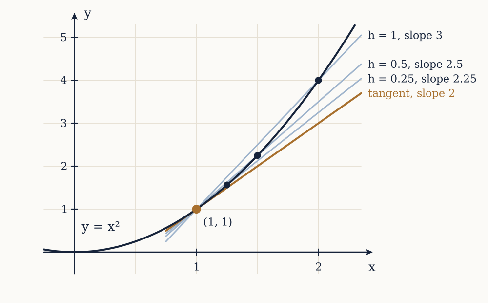
The obvious repair is to use a second point nearby and accept a small error. Take the point at $x=1$, where $y=1$, and a second at $x=1+h$, where $y=(1+h{)}^2$. The line through the two, a secant, has slope

which for $h=0.1$ is $2.1$, for $h=0.01$ is $2.01$, and for $h=0.001$ is $2.001$. Coming in from the other side, $h=-0.001$ gives $1.999$. The numbers are converging on $2$ from both directions and never reaching it, and the one value of $h$ that would give the slope at the point itself, $h=0$, turns the fraction into $0/0$ and says nothing at all.

Something is clearly true here: the numbers are closing in on $2$ and would go on closing in forever. Saying what that means, precisely enough to calculate with, is the whole of the next lesson.

Example. Estimate the slope of $y=x^3$ at $x=2$ using secants.

With $h=0.1$ the second point is $x=2.1$, where $y=9.261$, so the secant slope is $(9.261-8)/0.1=12.61$. With $h=0.01$ the point is $x=2.01$, where $y=8.120601$, giving $(8.120601-8)/0.01=12.0601$. With $h=0.001$ the slope is $12.006001$. The values are converging on $12$, and every one of them is an honest slope of an honest line, none of which is the tangent.

Now you. Estimate the slope of $y=1/x$ at $x=2$ with $h=0.1$, $h=0.01$ and $h=0.001$.

The area under a curve

The second problem is older. Areas bounded by straight lines are elementary: a rectangle is a product, a triangle is half of one, and any polygon can be cut into triangles. Curved boundaries defeat this completely, because no finite number of straight cuts will follow a curve.

Take the region under $y=x^2$ from $x=0$ to $x=1$. There is obviously an area there, somewhere between nothing and the unit square, but no formula in school geometry produces it. The available approximation is to fill the region with rectangles. Cut $[0,1]$ into four strips of width $1/4$ and give each rectangle the height of the curve at the right end of its strip: the heights are $(1/4{)}^2,(2/4{)}^2,(3/4{)}^2,(4/4{)}^2$, and the total area is $0.46875$. Do the same with the left end of each strip and the total is $0.21875$.

Those two numbers bracket the truth, because $x^2$ rises across the interval, so right ends overestimate and left ends underestimate. The bracket is embarrassingly wide. Going to ten strips narrows it to between $0.285$ and $0.385$; a hundred strips gives $0.32835$ to $0.33835$; a thousand gives $0.332834$ to $0.333834$. The gap is closing on zero and both ends are closing on $1/3$.

Again something is true and unstated. No finite number of rectangles ever gives the area, every one of them is wrong, and the sequence of wrong answers is unmistakably heading somewhere.

Example. Bracket the area under $y=x^2$ from $0$ to $1$ using five strips.

Each strip is $0.2$ wide. Right ends give heights $0.04,0.16,0.36,0.64,1$, summing to $2.2$, so the area estimate is $0.2\times 2.2=0.44$. Left ends give heights $0,0.04,0.16,0.36,0.64$, summing to $1.2$, for an estimate of $0.24$. The true area lies between them, and the width of the bracket, $0.2$, is exactly one strip width times the total rise of the function, which is a pattern worth remembering.

Now you. Bracket the area under $y=x^2$ from $0$ to $1$ using ten strips.

What Archimedes did about it

The area problem was solved, in particular cases, about nineteen centuries before calculus existed. Archimedes of Syracuse, working around 240 BC, computed the exact area of a parabolic segment: the region cut off from a parabola by a straight chord.

His construction inscribes the largest triangle in the segment, then the two largest triangles in the two gaps that remain, then four in the four gaps left by those, and so on. He proved geometrically that each generation of triangles has one quarter of the total area of the previous generation. The segment is therefore the first triangle multiplied by $1+1/4+1/16+1/64+\dots$, and that geometric series sums to $4/3$. The area of the segment is four thirds of the inscribed triangle, exactly, with no approximation surviving in the answer.

The same author bracketed $\pi$ in Measurement of a Circle by inscribing and circumscribing regular polygons of $96$ sides, obtaining $3\frac{10}{71}<\pi <3\frac{1}{7}$, which is $3.14085<\pi <3.14286$, against the true $3.14159$. The technique, called the method of exhaustion, is rigorous by any standard: to prove the area equals $A$, show that assuming it larger and assuming it smaller both lead to contradictions.

The trouble with exhaustion is that it is a proof technique, not a method of discovery. Each new region needs its own geometric argument, invented from nothing, and Archimedes needed to know the answer before he could prove it. Two thousand years produced only a handful of successes. What was missing was not rigour but a procedure.

The two problems are one

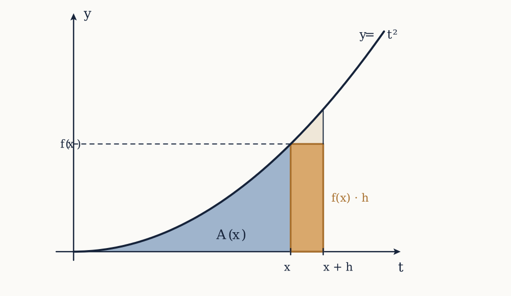
Here is the connection that makes a subject out of two puzzles, and it is easiest to see in physics. Let $s(t)$ be the distance a body has travelled by time $t$, and $v(t)$ its speed. If you plot $s$ against $t$, the slope at any instant is the speed at that instant: speed is a rate, and a rate is a slope. If instead you plot $v$ against $t$, the area under the graph up to time $t$ is the distance covered, since distance is speed accumulated over time.

So the slope problem takes position to speed, and the area problem takes speed back to position. They run in opposite directions between the same two quantities, which suggests they are inverse operations, and that whichever is easier to compute solves both.

A falling body makes the claim checkable. Near the Earth's surface a body released from rest falls with speed $v=9.8t$ metres per second after $t$ seconds, which plots as a straight line through the origin. The area under it from $0$ to $3$ seconds is a triangle of base $3$ and height $29.4$, so the area is $44.1$. The distance formula for constant acceleration, from mechanics, is $s=\frac{12}{g}{t}^2$, giving $\frac{12}{(}9.8)(9)=44.1$ metres. The area under the speed graph is the distance, to the last digit.

Example. Use the area under $v=9.8t$ to find the distance fallen in $5$ seconds, and check it.

The region is a triangle of base $5$ and height $9.8\times 5=49$, so the area is $\frac{12}{(}5)(49)=122.5$. The formula $s=\frac{12}{g}{t}^2$ gives $\frac{12}{(}9.8)(25)=122.5$ metres. They agree, and notice that the area calculation needed no formula for falling bodies: it read the answer off the graph.

Now you. A car accelerates from rest so that its speed is $v=4t$ metres per second. How far does it travel in the first $6$ seconds, and what is the slope of the distance graph at $t=6$?

Ghosts of departed quantities

Isaac Newton and Gottfried Wilhelm Leibniz, working independently in the 1660s and 1670s, each found the procedure that exhaustion lacked, and each published a calculus in which slopes and areas are computed by rules rather than reinvented per problem. Newton spoke of fluxions, rates at which quantities flow; Leibniz wrote $dx$ and $dy$ for infinitesimal differences and invented the notation still used today. The results were spectacular and immediately convincing, because they reproduced everything the ancients had done and much they had not.

The reasoning was not defensible. In a typical Leibnizian calculation, $dx$ is a quantity small enough that $(dx{)}^2$ may be discarded as negligible, and at the end of the calculation $dx$ is divided out, which requires it to be non-zero, and then dropped, which requires it to be zero. Bishop George Berkeley attacked exactly this in The Analyst of 1734, asking of the vanishing increments: "May we not call them the ghosts of departed quantities?" The complaint was fair, and no clean answer existed for almost a century.

The repair came from Augustin-Louis Cauchy, whose Cours d'Analyse of 1821 made the limit rather than the infinitesimal the basic notion, and from Karl Weierstrass, who in the 1860s gave the limit the tolerance-based definition that removes every appeal to intuition about the infinitely small. Nothing in the results changed. What changed is that the results acquired proofs.

Two remarks about that history are worth carrying forward. First, useful mathematics is regularly used for a century before it is made rigorous, so a working physicist's cheerful manipulation of $dx$ is not ignorance but inheritance. Second, the rigorous version is not decoration: without it there is no way to tell a valid infinitesimal argument from an invalid one, and both kinds were published.

What the rest of this course does

The plan follows the trouble. The immediate need is a precise account of what it means for the secant slopes to close in on $2$, which is the limit, and that occupies the next two lessons, since the limit also settles what it means for a function to have no breaks in it.

With limits available, the slope problem is solved in one definition and then made practical: a handful of rules reduce a page of limit algebra to a line, and by the middle of the course any function that can be written down can be differentiated. Those derivatives immediately answer questions that look nothing like slopes, from the maximum range of a projectile to the angle at which light bends entering water.

The area problem is then defined properly as a limit of rectangle sums, computed the hard way once, and after that the connection glimpsed above is proved as the Fundamental Theorem of Calculus. That theorem converts every area problem into the search for a function with a given derivative, which is what makes areas, volumes, work and averages computable at all.

The last lesson does the reverse trick: instead of computing exactly, it replaces a function by a polynomial that matches it near a point, which is where every approximation in a physics textbook comes from. Before any of that, a definition is owed.

The secant slopes of the previous lesson closed in on a number without ever reaching it, and that behaviour needs a definition before anything can be built on it.

The word usually offered is "approaches", which is a description rather than a definition: it says what the numbers are doing without saying what would settle whether a claimed answer is right. This lesson replaces it with something checkable, and then, having made limits precise, shows that most of them are computed in one step by substitution. The interesting ones are exactly the ones where substitution fails.

The tolerance game

Consider the claim that $f(x)=2+x$ approaches $2$ as $x$ approaches $0$. It is obviously true, but ask what makes it true and the answer is not "the values get near $2$", since the values also get near $2.0001$ and near $3$.

The claim that distinguishes $2$ from every other candidate is this: name any tolerance, however small, and I can keep $f(x)$ within it. Ask for $f(x)$ within $0.01$ of $2$ and I keep $x$ within $0.01$ of $0$. Ask for $0.000001$ and I keep $x$ within $0.000001$. No other number survives this game. If you propose $2.0001$ as the limit and I ask for a tolerance of $0.00001$, you cannot deliver, because once $x$ is small the values are nowhere near $2.0001$.

The limit is therefore not a description of motion but a guarantee about tolerances, and the guarantee has two players: a challenge, and a response that must exist for every challenge. Weierstrass turned exactly this into notation in the 1860s. Writing $\epsilon$ for the challenge tolerance on the output and $\delta$ for the response tolerance on the input,

means: for every $\epsilon >0$ there is a $\delta >0$ such that $0<|x-a|<\delta$ forces $|f(x)-L|<\epsilon$.

Two details in that sentence carry real weight. The order is fixed: $\epsilon$ is named first and $\delta$ may depend on it, never the reverse. And the condition on the input is $0<|x-a|$, which explicitly excludes $x=a$. The limit is a statement about the punctured neighbourhood of $a$, and it is deliberately blind to the value of $f$ at $a$, which may be anything or may not exist. That blindness is not a technicality: it is the only reason the definition is usable for difference quotients, which are always undefined at the point of interest.

Producing a delta

The definition earns its keep when a $\delta$ is actually produced, so here is one. Claim: $\underset{x\to 3}{lim}(4x-5)=7$. Given $\epsilon$, the requirement is $|(4x-5)-7|<\epsilon$, which is $|4x-12|<\epsilon$, which is $4|x-3|<\epsilon$. So taking $\delta =\epsilon /4$ works, for every $\epsilon$ at once. The proof is the formula for $\delta$.

A curve needs one extra move. Claim: $\underset{x\to 2}{lim}{x}^2=4$. The quantity to control is $|x^2-4|=|x-2|\cdot |x+2|$. The first factor is what $\delta$ controls directly; the second must be bounded before it can be used. So agree in advance that $\delta$ will never exceed $1$, which confines $x$ to the interval from $1$ to $3$ and makes $|x+2|<5$. Then $|x^2-4|<5|x-2|<5\delta$, so choosing $\delta$ to be whichever of $1$ and $\epsilon /5$ is smaller finishes it.

Check it numerically with $\epsilon =0.05$, which gives $\delta =0.01$. At $x=2.01$ the error is $|4.0401-4|=0.0401$, and at $x=1.99$ it is $0.0399$. Both are under the requested $0.05$, with room to spare, which is normal: $\delta$ has to work, not to be optimal.

Nobody computes everyday limits this way, any more than anyone adds by returning to the axioms of arithmetic. The definition is there so that the shortcuts can be proved, and so that a disputed limit has a court of appeal.

The limit laws, and why substitution usually works

From the definition it can be proved, once and for all, that limits respect arithmetic. If $\underset{x\to a}{lim}f(x)=L$ and $\underset{x\to a}{lim}g(x)=M$, then the limit of $f+g$ is $L+M$, of $f-g$ is $L-M$, of $fg$ is $LM$, and of $f/g$ is $L/M$ provided $M\ne 0$. Constants pull out, and powers and roots behave as expected.

Add the two limits that are true directly from the definition, $\underset{x\to a}{lim}c=c$ and $\underset{x\to a}{lim}x=a$, and a large class of limits collapses. A polynomial is built from constants and $x$ by multiplication and addition, so for any polynomial $P$, $\underset{x\to a}{lim}P(x)=P(a)$: substitute and stop. A rational function is a quotient of polynomials, so the same holds wherever the denominator is not zero at $a$.

That is the useful summary. For every function assembled by arithmetic from polynomials, the limit is the value, and the calculation is one substitution. So $\underset{x\to 2}{lim}(x^3-4x+1)=8-8+1=1$, and there is nothing more to say about it.

The whole subject therefore lives in the exceptions, and there is essentially one: the denominator goes to zero at the same moment as the numerator. The law for quotients does not apply, the expression $0/0$ is not defined, and yet the limit frequently exists. Such an expression is called an indeterminate form, and the name is precise. It is not that the answer is unknown; it is that the form itself determines nothing, since $0/0$ arises in limits equal to $6$, to $0$, to $-1/4$ and to nothing at all.

Working the indeterminate forms

The technique is always the same: change the expression algebraically so that the cancellation happens before the limit is taken. This is legitimate because the limit ignores the point itself, so any manipulation valid for $x\ne a$ is valid here even if it is invalid at $a$.

For $\underset{x\to 3}{lim}\frac{x^2-9}{x-3}$, substitution gives $0/0$. Factor: $x^2-9=(x-3)(x+3)$, so for every $x\ne 3$ the expression equals $x+3$, and the limit is $6$. The cancelled factor is the whole difficulty, and cancelling it is legal for exactly the values the limit is about.

Example. Evaluate $\underset{x\to 2}{lim}\frac{x^3-8}{x-2}$.

Substitution gives $0/0$, so factor the numerator: $x^3-8=(x-2)(x^2+2x+4)$, which the factor theorem from the previous course guarantees since $x=2$ is a root. For $x\ne 2$ the quotient is $x^2+2x+4$, a polynomial, so the limit is $4+4+4=12$. Numerically, at $x=2.001$ the original expression is $12.006$, which agrees.

Now you. Evaluate $\underset{x\to 1}{lim}\frac{x^3-1}{x^2-1}$.

Roots need a different device: multiply by the conjugate, which moves the difficulty from the numerator to the denominator where it does no harm.

Example. Evaluate $\underset{h\to 0}{lim}\frac{\sqrt{9+h}-3}{h}$.

Multiply top and bottom by $\sqrt{9+h}+3$. The numerator becomes $(9+h)-9=h$, so the expression is $h/[h(\sqrt{9+h}+3)]$, which for $h\ne 0$ is $1/(\sqrt{9+h}+3)$. Now substitution is legal and gives $1/6=0.1667$. Checking with $h=0.001$ in the original gives $0.166662$, so the algebra and the arithmetic agree.

Now you. Evaluate $\underset{h\to 0}{lim}\frac{\sqrt{4+h}-2}{h}$.

Both of those are difference quotients in disguise, which is the point. The limit machinery was invented for them.

When there is no limit

A limit can fail to exist, and the ways it fails are worth knowing by sight, because a rule applied to a limit that does not exist produces confident nonsense.

The commonest failure is a jump: the two sides disagree. For $f(x)=|x|/x$, every positive $x$ gives $+1$ and every negative $x$ gives $-1$. Approaching zero from the right the values sit at $1$, from the left at $-1$, and no single number is being approached. This motivates one-sided limits, written $\underset{x\to a^{+}}{lim}$ and $\underset{x\to a^{-}}{lim}$, with the obvious definitions restricted to one side. The two-sided limit exists exactly when both one-sided limits exist and are equal, which is a theorem, and it is the standard way to test a function defined by different formulas on either side of a point.

The second failure is blowing up. For $f(x)=1/x^2$ near zero the values exceed any bound you name. Writing $\underset{x\to 0}{lim}1/x^2=\infty$ is standard and convenient, but it does not assert that the limit exists: it is shorthand for a specific mode of not existing, namely that the values eventually exceed every fixed number. Treating that $\infty$ as a quantity to cancel or divide by is how people prove that $1=2$.

The third failure is oscillation. As $x$ approaches zero, $\sin (1/x)$ runs through every value between $-1$ and $1$ infinitely often, no matter how small an interval around zero you take. Nothing is approached, nothing blows up, and no tolerance smaller than $1$ can ever be met.

Limits at infinity, and squeezing

Reversing the roles of the two tolerances gives the other kind of limit. Saying $\underset{x\to \infty }{lim}f(x)=L$ means: name any $\epsilon$, and there is a value of $x$ beyond which $f$ stays within $\epsilon$ of $L$. The graph of such a function has a horizontal asymptote at height $L$.

For rational functions these limits are settled by dividing top and bottom by the highest power present. Take $(3x^2+2x-1)/(5x^2-x+4)$ and divide through by $x^2$ to get $(3+2/x-1/x^2)/(5-1/x+4/x^2)$. Every term with an $x$ downstairs vanishes, so the limit is $3/5$. The arithmetic bears this out: at $x=10$ the value is $0.6457$, at $x=100$ it is $0.60514$, and at $x=1000$ it is $0.60052$.

Example. Evaluate $\underset{x\to \infty }{lim}\frac{2x^3-x}{6x^3+5}$.

Divide by $x^3$: the expression becomes $(2-1/x^2)/(6+5/x^3)$, and the limit is $2/6=1/3$. At $x=100$ the original is $0.333316$, closing on $0.3333$ from below.

Now you. Evaluate $\underset{x\to \infty }{lim}\frac{4x^2+7}{x^3-2}$.

One further tool is needed later and is easiest to state now. The squeeze theorem says that if $g(x)\le f(x)\le h(x)$ near $a$, and $g$ and $h$ both have limit $L$ at $a$, then $f$ does too: a function trapped between two things converging to the same place has nowhere else to go.

Its standard use is $f(x)=x^2\sin (1/x)$ near zero. The oscillating factor never leaves $[-1,1]$, so $-x^2\le f(x)\le x^2$, and both bounds go to zero. Hence $f(x)\to 0$, despite oscillating infinitely often on the way. The values confirm it: at $x=0.01$ the function is about $-5.06\times {10}^{-5}$, and at $x=0.001$ about $8.27\times {10}^{-7}$. This theorem is what will deliver the derivative of the sine function, where no algebraic trick works at all.

What has been bought

The limit is now a definition rather than a gesture, and with the limit laws most limits are one substitution. The exceptions are the indeterminate forms, and the two shown here, factoring and rationalising, handle a large fraction of what the next lessons produce.

Notice what has been carefully avoided throughout: any claim about $f(a)$. The limit at $a$ can exist while $f(a)$ is undefined, as in every difference quotient, or while $f(a)$ is defined and equal to something else entirely, if the function is given a stray value at one point. Functions where nothing so perverse happens, where the limit is the value, are the ones on which the rest of the subject is built, and they have a name and a set of theorems of their own.

A limit at a point is deliberately blind to the value of the function at that point, and the functions worth working with are precisely the ones where that blindness costs nothing.

The previous lesson built the limit as a promise about tolerances and showed that for polynomials and similar functions the limit is just the value, so the whole calculation is a substitution. That coincidence deserves a name and an investigation, because it is not automatic, and because the theorems that follow from it are what later lessons quietly rely on when they assert that a maximum exists or that an area is a number.

The definition, in three parts

A function $f$ is continuous at $a$ when

and that single equation is really three demands stacked together. The right side must exist, so $a$ must be in the domain of $f$. The left side must exist, so the function must approach some single value from both sides. And the two must be equal.

Any one of the three can fail on its own. The function $(x^2-9)/(x-3)$ has a perfectly good limit of $6$ at $x=3$ and no value there at all. A function defined to be $x^2$ everywhere except at $x=1$, where it is declared to be $7$, has both a limit ($1$) and a value ($7$), and they disagree. A step function has a value at the step and no limit.

The picture everyone is taught, that a continuous function can be drawn without lifting the pen, is a decent guide and a poor definition. It fails to say anything useful about a function on the rationals, or about $\sin (1/x)$, which cannot be drawn at all near zero yet is continuous at every point where it is defined. The tolerance definition survives all such cases, which is why it is the one that is used.

A function is continuous on an interval when it is continuous at every point of it, with the endpoints requiring only the one-sided limit that stays inside.

Example. For which value of $c$ is the function equal to $x^2$ when $x\le 2$ and to $cx+1$ when $x>2$ continuous everywhere?

Away from $x=2$ each piece is a polynomial and so is continuous. At $x=2$ the value and the limit from the left are both $4$. The limit from the right is $2c+1$. Continuity requires $2c+1=4$, so $c=1.5$. With that choice the right-hand formula at $x=2$ gives $1.5\times 2+1=4$, matching, and the graph has no step in it.

Now you. The function equals $(x^2-25)/(x-5)$ for $x\ne 5$ and equals $k$ at $x=5$. What $k$ makes it continuous?

The three ways it fails

Discontinuities come in a small number of shapes, and naming them is useful because the repair, if any, differs.

A removable discontinuity is a hole: the limit exists but the value is missing or wrong. It is removable in the literal sense that redefining the function at that one point fixes it, which is what the previous exercise did. Every cancelled factor in an indeterminate form leaves one of these behind.

A jump discontinuity is two one-sided limits that exist and disagree. These are not repairable by any single value, and they are common in real data rather than pathological: a postage rate as a function of weight, an income tax rate as a function of income, the density of water as a function of temperature at 0 degrees Celsius. Physical laws are usually written for continuous quantities, and a jump is where such a law needs separate treatment on each side.

An infinite discontinuity is a vertical asymptote, as in $1/x$ at zero, where no value assigned at the point can help because the function is unbounded nearby. Oscillation, as in $\sin (1/x)$ at zero, is the remaining case and is equally unrepairable.

Example. Classify the discontinuities of $f(x)=\frac{x^2-x-6}{x^2-9}$.

The denominator vanishes at $x=3$ and $x=-3$, so those are the only candidates. Factoring gives $(x-3)(x+2)$ over $(x-3)(x+3)$, so for $x\ne 3$ the function equals $(x+2)/(x+3)$. At $x=3$ that expression is $5/6=0.8333$, a perfectly good limit with no value attached, so the discontinuity is removable. At $x=-3$ the reduced form still has a zero denominator with a non-zero numerator, so the function blows up: an infinite discontinuity, and no redefinition will fix it.

Now you. Classify the discontinuities of $f(x)=\frac{x^2-1}{x^2-3x+2}$.

Almost everything is continuous

The limit laws convert directly into a catalogue. Sums, differences, products and quotients of continuous functions are continuous wherever they are defined, and so is a composition of continuous functions. Polynomials are continuous everywhere. Rational functions are continuous except where the denominator vanishes. Roots, sines, cosines, exponentials and logarithms are continuous throughout their domains.

The practical consequence is that continuity is the default. Any function written down by combining the standard ones is continuous except at points you can find by inspection: division by zero, an even root of a negative number, a logarithm of something non-positive, or a definition given in pieces. Everything else is safe.

That fact is what makes the next two theorems worth having. They are hypotheses-and-conclusion statements whose hypothesis is almost always satisfied, so in practice they hand out conclusions for free.

A sign change guarantees a root

The Intermediate Value Theorem says that if $f$ is continuous on the closed interval from $a$ to $b$, then $f$ takes every value between $f(a)$ and $f(b)$ somewhere in that interval. In particular, if $f(a)$ and $f(b)$ have opposite signs, there is a point where $f$ is zero.

It sounds like a restatement of the pen-drawing picture, and it is much more than that: it is an existence theorem that converts a comparison of two numbers into a guarantee about the existence of a solution. It says nothing about where the root is or how many there are, and it needs no formula for solving anything.

Turned into a procedure, it gives bisection. Take $f(x)=x^3-x-1$, which no factoring will crack since it has no rational roots. Then $f(1)=-1$ and $f(2)=5$, so a root exists between $1$ and $2$. Evaluate at the midpoint: $f(1.5)=0.875$, positive, so the sign change is now between $1$ and $1.5$. Then $f(1.25)=-0.296875$, so the root is between $1.25$ and $1.5$. Then $f(1.375)=0.224609$, then $f(1.3125)=-0.051514$, then $f(1.34375)=0.082611$, then $f(1.328125)=0.014576$. Six steps have trapped the root between $1.3125$ and $1.328125$, and each further step halves the interval. The root, to seven figures, is $1.324718$.

Bisection is slow and utterly reliable: the error is guaranteed to fall by half per step, so twenty steps take an interval of width one down to below a millionth. Later in the course a much faster method appears, one that uses derivatives and can fail, and the comparison between them is the usual trade in numerical work.

Example. Show that $\cos x=x$ has a solution between $0$ and $1$, and bracket it in three bisection steps.

Apply the theorem to $g(x)=\cos x-x$, which is continuous everywhere. Here $g(0)=1$ and $g(1)=0.5403-1=-0.4597$, opposite signs, so a solution exists. The midpoint gives $g(0.5)=0.377583$, so the root lies in $[0.5,1]$. Then $g(0.75)=-0.018311$, so it lies in $[0.5,0.75]$. Then $g(0.625)=0.185963$, so it lies in $[0.625,0.75]$. The true value is $0.739085$.

Now you. Show that $x^3=10$ has a solution between $2$ and $3$, and take two bisection steps.

Why the theorem needs the real numbers

The Intermediate Value Theorem is not a triviality, and the cleanest evidence is that it is false if the number system has gaps.

Work entirely within the rational numbers and consider $f(x)=x^2-2$. It is continuous as a function of a rational variable, $f(1)=-1$, and $f(2)=2$. The signs are opposite, yet there is no rational number where $f$ is zero, since the previous course proved by contradiction that $\sqrt{2}$ is irrational. Continuity and a sign change are not enough. What is also needed is that the line has no holes in it.

That property, called completeness, is the defining difference between the rationals and the reals, and every existence theorem in this course descends from it. Continuity is the hypothesis you check; completeness is the hypothesis that comes with the number system and is easy to forget. Cauchy, Weierstrass, Dedekind and Cantor spent the middle of the nineteenth century making it precise, and calculus was placed on solid ground only when they had.

A closed interval guarantees a maximum

The second existence theorem is the Extreme Value Theorem: a continuous function on a closed bounded interval attains a maximum and a minimum somewhere on it. Not approaches, attains, at actual points of the interval.

Both hypotheses are load-bearing, and dropping either kills the conclusion. The function $1/x$ on the half-open interval $(0,1]$ is continuous there and has no maximum, since it exceeds any bound near zero. The function $f(x)=x$ on the open interval $(0,1)$ is continuous and bounded, and still has no maximum: it gets arbitrarily close to $1$ and never attains it, and no point of the interval is the winner. Take the same function on the closed interval $[0,1]$ and the maximum exists, at the endpoint. And a function with a jump can miss its own supremum even on a closed interval.

This theorem is the licence for the whole optimisation lesson later. When a problem asks for the shape that minimises cost, the answer is presumed to exist, and this is where that presumption comes from: continuous function, closed interval, therefore a minimum exists, and the derivative can then be used to find where it is. Without the theorem, the derivative would only be able to say that if a minimum exists then it is at one of these points.

Continuity is not enough for a tangent

Continuity guarantees no holes, no jumps and no blowups. It does not guarantee that a curve has a direction at each point, and that gap is what the next lesson has to close.

The function $f(x)=|x|$ is continuous everywhere, including at zero, where the limit and the value are both zero. But it has a corner there. Approach the origin along the left branch and the slope is $-1$; approach along the right branch and it is $+1$. Any line through the origin is a bad fit to at least one side, and there is no sensible tangent. The secant slopes from the previous lesson do exist here, but the one-sided limits disagree, which is exactly the jump failure applied to the difference quotient rather than to the function.

How much worse this can get was settled by Weierstrass in 1872, when he exhibited a function continuous at every point of the real line and differentiable at none. It is built as an infinite sum of ever faster, ever smaller cosine waves, so that at every scale, no matter how far you zoom in, the graph is still wrinkled and never settles down to look like a line. Until then most mathematicians assumed a continuous function must have a tangent almost everywhere, and the example ended that assumption permanently. It also demonstrates that intuition about curves is not a reliable guide, which is a large part of why the tolerance definitions were adopted.

So a curve can be unbroken and still have no slope. Having a slope at a point is a strictly stronger condition, and defining it, computing it and using it is what the next several lessons are about.

The slope of a curve at a single point can now be defined, because the limit supplies exactly the missing idea: the tangent slope is the number the secant slopes close in on.

Everything in this lesson comes from one formula, applied patiently. The earlier lessons supply the two things it needs: a definition of the limit as a promise about tolerances, and the warning from continuity that some curves have no slope at some points, so the definition must be allowed to fail rather than being assumed to work.

The definition

Fix a point $a$ in the domain of $f$. A second point at horizontal distance $h$ gives the secant slope

which is an ordinary quotient of ordinary numbers for every $h\ne 0$, and is undefined at $h=0$. The derivative of $f$ at $a$ is the limit of that quotient as $h$ approaches zero:

When the limit exists, $f$ is differentiable at $a$ and $f^{\prime }(a)$ is the slope of the tangent line there. When it does not, $f$ has no derivative at $a$, and this happens often enough that the qualification matters.

An equivalent form replaces $a+h$ by a variable point $x$, giving $f^{\prime }(a)=\underset{x\to a}{lim}(f(x)-f(a))/(x-a)$. The two are the same statement with different bookkeeping, and both are used: the first is easier to compute with, the second easier to reason with.

Note where the difficulty went. The expression is $0/0$ at $h=0$, which is why no algebraic evaluation is possible and why the limit is indispensable. Every derivative computed from the definition is an indeterminate form resolved by the techniques of the limits lesson, and in practice the resolution is nearly always the same: cancel an $h$ that appears in every term of the numerator.

Three derivatives from first principles

Take $f(x)=x^2$. The numerator is $(x+h{)}^2-x^2=2xh+h^2$, so the quotient is $(2xh+h^2)/h$, which for $h\ne 0$ equals $2x+h$. That is a polynomial in $h$, so the limit is a substitution: $f^{\prime }(x)=2x$. At $x=1$ this gives $2$, which is the number the secants of the first lesson were closing on.

Take $f(x)=1/x$, with $x\ne 0$. The numerator is $\frac{1}{x+h}-\frac{1}{x}=\frac{x-(x+h)}{x(x+h)}=\frac{-h}{x(x+h)}$. Dividing by $h$ gives $-1/[x(x+h)]$, and now substitution is legal: $f^{\prime }(x)=-1/x^2$. At $x=2$ that is $-0.25$, matching the secant values of $-0.238$ and $-0.2488$ computed earlier for $h=0.1$ and $h=0.01$. The sign is negative everywhere, as it must be for a function that falls on both branches.

Take $f(x)=\sqrt{x}$, with $x>0$. Here the trick is the conjugate. Multiplying the quotient above and below by $\sqrt{x+h}+\sqrt{x}$ turns the numerator into $(x+h)-x=h$, so the quotient becomes $1/(\sqrt{x+h}+\sqrt{x})$, and the limit is

At $x=9$ that is $1/6=0.16667$, and the secant with $h=0.001$ gives $0.166662$. Notice the behaviour near zero: as $x$ shrinks the derivative grows without bound, which is the graph turning vertical at the origin.

Example. Differentiate $f(x)=x^2-5x$ from the definition and find the slope at $x=1$.

The numerator is $[(x+h{)}^2-5(x+h)]-[x^2-5x]=2xh+h^2-5h$. Every term carries an $h$, so dividing gives $2x+h-5$, and the limit as $h\to 0$ is $f^{\prime }(x)=2x-5$. At $x=1$ the slope is $-3$: the curve is falling there, which is right, since the vertex of this parabola sits at $x=2.5$.

Now you. Differentiate $f(x)=3x^2+2$ from the definition.

A function, not a number

In each of those calculations the answer came out as a formula in $x$ rather than a single value, which is the step that makes calculus a machine rather than a collection of measurements. The derivative function $f^{\prime }$ assigns to each point where $f$ is differentiable the slope of $f$ there, and it has its own domain, its own graph, and its own derivative.

That last remark gives the second derivative $f^{\prime \prime }$, the rate at which the slope itself is changing. For $f(x)=x^2$ the derivative is $2x$ and the second derivative is the constant $2$: the slope increases at a steady rate, which is exactly what a parabola opening upward looks like. Third and higher derivatives follow by repetition, and the notation $f^{(4)}$ takes over once primes become unreadable.

The physical reading is worth fixing now because the whole of mechanics uses it. If $s(t)$ is position, then $s^{\prime }(t)$ is velocity and $s^{\prime \prime }(t)$ is acceleration. Newton's second law, $F=ma$, is therefore a statement about a second derivative, which is why the equations of physics are differential equations and why this course is a prerequisite for reading them.

Two notations

Lagrange's notation, $f^{\prime }(x)$, is compact and treats the derivative as an operation producing a new function. It is best when the functions are the objects of interest.

Leibniz's notation writes the same thing as

which records more. It names both variables, so in a problem with several it is unambiguous which is varying with respect to which. It carries the units correctly: if $y$ is in metres and $x$ in seconds, the symbol reads as metres per second without any further convention, and a derivative of position with respect to time therefore has units of m s⁻¹ while its own derivative has m s⁻². And it survives the chain rule in a form that looks like cancelling fractions, which is the main reason physicists use it and the main reason it must be handled with care: $dy/dx$ is a single symbol, the limit of a ratio, not a ratio of two quantities called $dy$ and $dx$. The nineteenth century spent considerable effort removing the implication that it is, and the notation kept the shape anyway because the shape is a good mnemonic.

A value at a specific point is written $f^{\prime }(3)$ in one notation and, less gracefully, as $dy/dx$ evaluated at $x=3$ in the other. Time derivatives in mechanics often use Newton's dot, $\dot{x}$ and $\ddot{x}$, which is unbeatable for brevity when the independent variable is always time.

Example. A stone falls from rest, so its distance fallen is $s=4.9t^2$ metres after $t$ seconds. Find its velocity at $t=2$ from the definition.

The difference quotient is $[4.9(2+h{)}^2-4.9(4)]/h=[19.6h+4.9h^2]/h=19.6+4.9h$, so the limit is $19.6$ metres per second. Numerically the quotient at $h=0.1$ is $20.09$, at $h=0.01$ it is $19.649$, and at $h=0.001$ it is $19.6049$, closing on $19.6$ exactly as the algebra says.

Now you. For the same stone, find the velocity at $t=3$, and the acceleration.

Differentiable implies continuous

There is one implication between the two conditions, and it goes one way only.

Suppose $f$ is differentiable at $a$. For $x\ne a$ write the identity

which is true because the fraction has been multiplied by what was just divided out. Take the limit as $x\to a$. The first factor tends to $f^{\prime }(a)$, a finite number, by assumption. The second tends to zero. By the product law the whole right side tends to $f^{\prime }(a)\cdot 0=0$, so $f(x)\to f(a)$, which is the definition of continuity at $a$.

So differentiability is the stronger condition, and the intuition matches: a function with a jump has a difference quotient that blows up across the jump, since a non-zero numerator is divided by a vanishing denominator.

The converse fails, and the previous lesson has already met the counterexample. For $f(x)=|x|$ at zero the difference quotient is $|h|/h$, which is $+1$ for positive $h$ and $-1$ for negative $h$. Both one-sided limits exist and disagree, so there is no derivative, while the function is perfectly continuous. The graph has a corner.

Two other failures are worth recognising by their difference quotients. For $f(x)=x^{1/3}$ at zero the quotient is $h^{1/3}/h=h^{-2/3}$, which grows without bound from both sides: the tangent is vertical, and a vertical line has no slope. For $f(x)=x^{2/3}$ at zero the quotient is $h^{-1/3}$, which goes to $+\infty$ from the right and $-\infty$ from the left: a cusp, where the curve comes to a point. In every case the diagnosis is the same, that the limit defining the derivative fails to exist, and the cases differ only in how it fails.

Reading a derivative

Once $f^{\prime }$ is available as a function, three features of it describe $f$ completely enough to sketch it.

The sign says direction. Where $f^{\prime }>0$ the tangent lines slope up and the function is increasing; where $f^{\prime }<0$ it is decreasing. This is the fact that makes derivatives useful for finding maxima, and it is stated here as a plausible reading rather than a theorem, because proving it needs the Mean Value Theorem, which arrives in a few lessons.

The magnitude says steepness, in the units of the problem. A derivative of $-0.25$ for $1/x$ at $x=2$ says that increasing $x$ by a small amount $\Delta x$ decreases $y$ by about $0.25\Delta x$. At $x=0.5$ the derivative is $-4$, sixteen times steeper, which is the same curve behaving very differently at a different place.

Example. For $f(x)=1/x$, find $f^{\prime }(0.5)$ and use it to estimate $f(0.51)$.

The derivative is $-1/x^2$, so $f^{\prime }(0.5)=-1/0.25=-4$. A step of $0.01$ in $x$ should therefore change $y$ by about $-4\times 0.01=-0.04$, predicting $f(0.51)\approx 2-0.04=1.96$. The true value is $1/0.51=1.960784$, so the prediction is right to three decimal places, and it was made without evaluating the function at the new point.

Now you. For $f(x)=x^3$, whose derivative is $3x^2$, estimate $f(2.01)$ from the value and derivative at $x=2$.

A zero says flat. At a point where $f^{\prime }(a)=0$ the tangent is horizontal, which happens at the top of a hill, the bottom of a valley, and also at neither, as at $x=0$ on $y=x^3$, where the curve merely pauses on its way up. Distinguishing those cases is the business of a later lesson.

What this costs, and what comes next

Every derivative in this lesson was computed by expanding a difference, cancelling an $h$, and taking a limit, and each took a paragraph. That is unsustainable. There is no chance of differentiating $(3x^2+1{)}^{10}/\sqrt{x^2+4}$ this way, and even $x^7$ requires the binomial expansion to be written out.

There is also a strong hint that no such labour should be necessary, because the answers are suspiciously tidy: $x^2$ gives $2x$, $x^3$ gives $3x^2$, $x^{1/2}$ gives ${\frac{12}{x}}^{-1/2}$, and $x^{-1}$ gives $-x^{-2}$. In every case the exponent has come down as a multiplier and dropped by one. If that pattern is genuine, and if the derivative of a sum, a product and a composition can be expressed in terms of the derivatives of the parts, then differentiation becomes mechanical and the limit definition retires to the role of justifying the rules.

That is exactly what happens, and the next lesson derives each rule from the definition rather than quoting it, because a rule whose derivation you have seen is a rule you can repair when you misremember it.

Differentiating from the definition costs a paragraph of algebra per function, and the answers are tidy enough to suggest that most of that work is repeated in the same way each time.

This lesson extracts the repetition into four rules. Each is proved from the difference quotient of the previous lesson, because a rule you have seen derived is one you can rebuild when memory garbles it, and because two of the four have plausible wrong versions that a derivation immediately kills. After this, the limit definition retires: it stays as the justification and stops being a method.

Linearity

Start with the two easiest. If $f$ and $g$ are differentiable, so is $f+g$, and $(f+g{)}^{\prime }=f^{\prime }+g^{\prime }$. The proof is one line of rearrangement: the difference quotient of $f+g$ is

and the limit of a sum is the sum of the limits, which is one of the limit laws. Similarly $(cf{)}^{\prime }=c{f}^{\prime }$ for a constant $c$, since the constant factors out of the quotient and then out of the limit.

Together these say that differentiation is linear, which is the property that lets a polynomial be differentiated term by term. It is worth noticing what is not claimed, because the pattern does not continue: there is no rule saying the derivative of a product is the product of the derivatives, and the next section shows why in one line.

A constant function has derivative zero, since every difference in the numerator is zero before any limit is taken. Geometrically it is a horizontal line, and the consequence for later work is that adding a constant to a function never changes its derivative, so a derivative cannot possibly determine its function uniquely.

The power rule

The pattern noticed at the end of the previous lesson, that $x^n$ differentiates to $n{x}^{n-1}$, can be proved for every positive integer $n$ using a factorisation from the earlier course:

Use the second form of the definition, with the quotient $(f(x)-f(a))/(x-a)$. The factor $(x-a)$ cancels exactly, leaving the long bracket, which is a polynomial and so may be evaluated at $x=a$ by substitution. Every one of its terms becomes $a^{n-1}$, and there are $n$ of them, so the limit is $n{a}^{n-1}$. Since $a$ was arbitrary, $f^{\prime }(x)=n{x}^{n-1}$ everywhere.

That covers positive integers. The quotient rule below extends it to negative integers, and the lesson on implicit differentiation extends it to every rational exponent; the result is the same formula in all cases, and it holds for irrational exponents too. So $x^7$ differentiates to $7x^6$, which at $x=2$ is $448$, and $\sqrt{x}=x^{1/2}$ differentiates to ${\frac{12}{x}}^{-1/2}$, agreeing with the conjugate calculation done from scratch earlier.

With linearity, every polynomial is now immediate. The derivative of $3x^4-5x^2+7x-2$ is $12x^3-10x+7$, written down in one pass with no limits anywhere.

The product rule

The plausible guess is $(fg{)}^{\prime }=f^{\prime }{g}^{\prime }$, and it is wrong. Test it on $f(x)=g(x)=x$: the product is $x^2$, whose derivative is $2x$, while the product of the derivatives is $1$. A rule that fails on the simplest possible case needs no further refutation. Leibniz himself conjectured the product of the differentials in his early notes in 1675 and corrected it within days, which is a good indication that the correct rule is not obvious.

Here is the derivation. The numerator of the difference quotient is $f(x+h)g(x+h)-f(x)g(x)$, and the trick is to add and subtract a hybrid term, $f(x+h)g(x)$, which changes nothing and splits the difference into two differences that each move only one factor:

Group the first pair and the second pair, divide by $h$, and the quotient becomes

Now take the limit. The two quotients tend to $g^{\prime }(x)$ and $f^{\prime }(x)$. The stray factor $f(x+h)$ tends to $f(x)$, and it does so because $f$ is differentiable and therefore continuous, which is where that theorem from the previous lesson earns its place. The result is

The rule is symmetric, which is a useful check, and it explains the failed guess: the true derivative has two terms because a product can change by either factor moving, and $f^{\prime }{g}^{\prime }$ counts neither of them.

Example. Differentiate $(x^2+1)(x^3-2x)$ and evaluate the derivative at $x=2$.

With $f=x^2+1$ and $g=x^3-2x$, the derivatives are $f^{\prime }=2x$ and $g^{\prime }=3x^2-2$. The rule gives $2x(x^3-2x)+(x^2+1)(3x^2-2)$. At $x=2$ the first term is $4\times 4=16$ and the second is $5\times 10=50$, so the derivative is $66$. Check by expanding first: the product is $x^5-x^3-2x$, whose derivative is $5x^4-3x^2-2$, giving $80-12-2=66$. The two routes agree, as they must.

Now you. Differentiate $(2x-1)(x^2+3)$ and evaluate at $x=1$.

The quotient rule

For a quotient the result is

valid wherever $g\ne 0$. It can be derived from the definition by the same add-and-subtract manoeuvre, but the quicker route is to write $q=f/g$, so that $f=qg$, and apply the product rule: $f^{\prime }=q^{\prime }g+q{g}^{\prime }$. Solving for $q^{\prime }$ gives $q^{\prime }=(f^{\prime }-q{g}^{\prime })/g$, and substituting $q=f/g$ and tidying over the common denominator produces the formula.

The minus sign and the order of the terms are the two things people get wrong, and the way to check them is a special case you already know. Take $f=1$ and $g=x$. The rule gives $(0\cdot x-1\cdot 1)/x^2=-1/x^2$, which matches the first-principles calculation of the derivative of $1/x$ done earlier. If a misremembered version gives $+1/x^2$, that test catches it at once.

The same special case extends the power rule downward. For $f=1$ and $g=x^n$ the rule gives $-n{x}^{n-1}/x^{2n}=-n{x}^{-n-1}$, which is the power rule with the exponent $-n$ in place of $n$. So the formula holds for negative integers too.

Example. Differentiate $\frac{x}{x^2+1}$ and evaluate at $x=2$.

Here $f=x$, $f^{\prime }=1$, $g=x^2+1$, $g^{\prime }=2x$. The rule gives $[(1)(x^2+1)-x(2x)]/(x^2+1{)}^2=(1-x^2)/(x^2+1{)}^2$. At $x=2$ that is $(1-4)/25=-0.12$. The sign is negative, and it should be: this function peaks at $x=1$ and declines thereafter, and the formula makes the peak visible, since the numerator $1-x^2$ vanishes exactly at $x=1$.

Now you. Differentiate $\frac{3x+1}{x-2}$ and evaluate at $x=3$.

The chain rule

The last rule is the one that matters most, because almost every function met in practice is a composition. Its statement, in Lagrange notation, is that if $y=f(u)$ and $u=g(x)$ then

or equivalently $(f\circ g{)}^{\prime }(x)=f^{\prime }(g(x))\cdot g^{\prime }(x)$: differentiate the outside function, leave the inside alone in it, and multiply by the derivative of the inside.

The reason it is a product is a statement about rates. If a car's fuel use rises by $3$ litres for each extra hour driven, and the cost rises by $1.60$ for each extra litre, then the cost rises by $4.80$ per extra hour, and the two rates multiply. The Leibniz form makes this look like cancellation of $du$, which is exactly why the notation was designed that way and exactly why the appearance is dangerous: the honest proof multiplies and divides by $\Delta u$, which is illegitimate whenever $\Delta u$ happens to be zero, and repairing that gap takes a page. The gap is real, the repair is standard, and the rule is true.

Example. Differentiate $\sqrt{x^2+9}$ and evaluate at $x=4$.

The outside function is $\sqrt{u}$, with derivative $1/(2\sqrt{u})$; the inside is $u=x^2+9$, with derivative $2x$. Multiplying gives $2x/(2\sqrt{x^2+9})=x/\sqrt{x^2+9}$. At $x=4$ the square root is $\sqrt{25}=5$, so the derivative is $4/5=0.8$. That number has a geometric meaning: this function is the distance from the origin to a point moving along a horizontal line nine units up, and $0.8$ is the component of the motion along the line of sight.

Now you. Differentiate $(x^3+1{)}^5$ and evaluate at $x=1$.

Compositions can be nested, and the rule composes with itself: each layer contributes its own derivative as a factor, working from the outside in. Differentiating $(3x^2+1{)}^{10}$ gives $10(3x^2+1{)}^9\cdot 6x$, and at $x=1$ that is $60\times 4^9=15\{,\}728\{,\}640$. The size of that number is a reminder that a modest-looking function can have an enormous rate of change, which is why exponents are where numerical trouble usually starts.

Assembling them

Real functions need several rules at once, and the only skill involved is deciding which structure is outermost before touching anything.

Take $y=\frac{x^2(2x+1{)}^3}{x-1}$. The outermost structure is a quotient, so the quotient rule applies with $f=x^2(2x+1{)}^3$ and $g=x-1$. Differentiating $f$ needs the product rule, with the second factor needing the chain rule: $f^{\prime }=2x(2x+1{)}^3+6x^2(2x+1{)}^2$. Assembling, $y^{\prime }=[f^{\prime }(x-1)-f]/(x-1{)}^2$. At $x=2$ the pieces are $f=4\times 125=500$ and $f^{\prime }=4\times 125+6\times 4\times 25=1100$, so $y^{\prime }=(1100\times 1-500)/1=600$.

The habit worth building is to name the pieces before differentiating anything, write the rule with the names, and only then substitute. Skipping that step is where the sign errors and the missing chain factors come from, and they come from it reliably.

Where the rules stop

Everything above is closed under the operations of algebra. Any function built from powers by adding, multiplying, dividing and composing can now be differentiated mechanically, and that class is large: all polynomials, all rational functions, all algebraic combinations of roots.

It does not include $\sin x$, and it does not include $2^x$. No amount of the power rule reaches them, because they are not built from powers by algebra: the sine is defined by a rotation and the exponential by repeated multiplication extended to the continuum. Their difference quotients lead to limits that no factoring or conjugate will resolve, in particular $\underset{h\to 0}{lim}(\sin h)/h$ and $\underset{h\to 0}{lim}(a^h-1)/h$.

Those two limits are the subject of the next lesson, and the second of them turns out to select a particular number as the natural base for an exponential, which is where $e$ actually comes from.

The rules of the previous lesson differentiate anything built from powers by algebra, and neither the sine nor an exponential is built that way, so each has to be taken back to the difference quotient.

What comes out is more interesting than a pair of formulas. The sine calculation only works in radians, and shows why. The exponential calculation produces a constant that depends on the base, and asking which base makes that constant equal to $1$ is where the number $e$ comes from, definitionally rather than as a decimal to memorise. This lesson assumes the unit circle definitions of sine and cosine and the exponential and logarithm laws from the earlier course.

Where the difference quotient leads

Apply the definition to $f(x)=\sin x$. The numerator is $\sin (x+h)-\sin x$, and the addition formula $\sin (x+h)=\sin x\cos h+\cos x\sin h$ turns it into $\sin x(\cos h-1)+\cos x\sin h$. Dividing by $h$ and grouping:

Both bracketed quotients are $0/0$ at $h=0$, and neither factors or rationalises. Neither depends on $x$, though, which is the important structural fact: two numbers settle the derivative of the sine at every point at once.

Numerically the two limits are not hard to guess. For $h=0.001$, $(\sin h)/h=0.99999983$ and $(1-\cos h)/h=0.0005$. So the candidates are $1$ and $0$, giving $\cos x$ as the derivative of $\sin x$. Guessing is not proving, and the first of the two needs a genuine argument.

The squeeze that settles $\sin h/h$

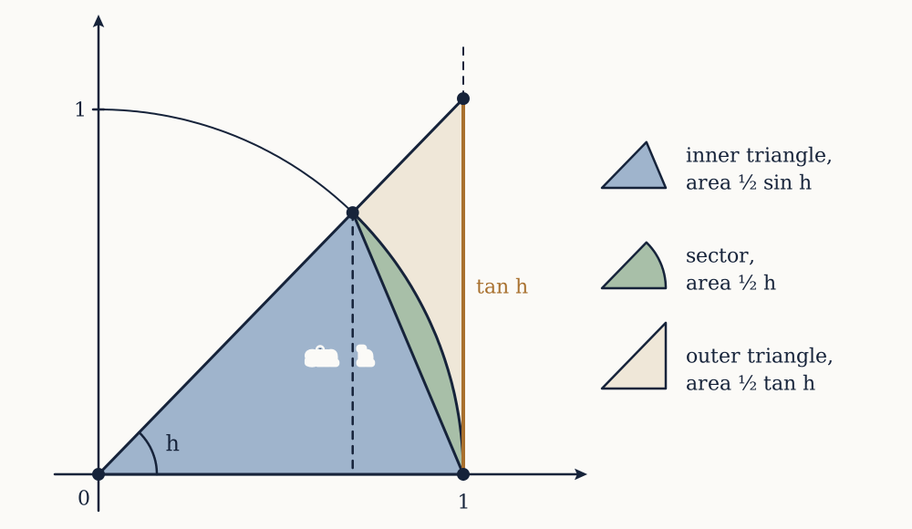
Take $h$ between $0$ and $\pi /2$ and draw the unit circle. Mark the angle $h$ at the centre, and compare three regions: the triangle with vertices at the centre, at the point $(1,0)$ and at the point on the circle; the circular sector between the same two radii; and the triangle formed by extending the radius to meet the tangent line at $(1,0)$.

Each region contains the previous one, so their areas are ordered. The first triangle has base $1$ and height $\sin h$, so its area is $\frac{12}{\sin }h$. The sector is the fraction $h/2\pi$ of the whole disc of area $\pi$, so its area is $\frac{12}{h}$: this is the step that requires $h$ to be measured in radians, since it is the radian measure that makes the arc length and the angle the same number. The outer triangle has base $1$ and height $\tan h$, so its area is $\frac{12}{\tan }h$. Therefore

Divide throughout by $\sin h$, which is positive, to get $1<h/\sin h<1/\cos h$, and invert to get $\cos h<(\sin h)/h<1$. As $h\to 0$ the left bound tends to $1$ because cosine is continuous, and the right bound is $1$. The squeeze theorem from the limits lesson does the rest:

The same holds from the negative side, since both $\sin h$ and $h$ change sign together and the quotient is unchanged.

The second limit now follows by the conjugate trick. Multiply $(1-\cos h)/h$ above and below by $1+\cos h$: the numerator becomes $1-{\cos }^{2}h={\sin }^{2}h$, so the quotient is $\frac{\sin h}{h}\cdot \frac{\sin h}{1+\cos h}$. The first factor tends to $1$ and the second to $0/2=0$, so the limit is $0$, confirming the numerical guess.

The radian requirement is not a formality. Measure angles in degrees and the sector area argument gives $h\pi /360$ instead of $h/2$, so the limit becomes $\pi /180=0.0174533$ and the derivative of the sine becomes $0.0174533\cos x$. That constant would then infest every formula in physics and engineering that involves an oscillation. Radians are used in calculus because they are the units in which this constant is $1$.

The derivatives of the trigonometric functions

Substituting the two limits into the grouped difference quotient gives, immediately,

with the second obtained the same way from the addition formula for cosine, and the minus sign coming from $\cos (x+h)=\cos x\cos h-\sin x\sin h$.

Differentiating repeatedly cycles with period four: sine goes to cosine, to minus sine, to minus cosine, and back. The consequence is that $y=\sin x$ satisfies

and so does $\cos x$, and so does any combination $A\sin x+B\cos x$. That equation is the mathematical content of simple harmonic motion: a mass on a spring obeys $F=-kx$, so by Newton's second law its acceleration is proportional to minus its displacement, which is this equation with a constant attached. The reason pendulums, tuning forks, LC circuits and molecular vibrations all produce sinusoids is that they all satisfy it.

The other trigonometric functions follow from the quotient rule. For $\tan x=\sin x/\cos x$,

which at $x=\pi /4$ equals $2$, since the cosine there is $1/\sqrt{2}$. The derivative is never less than $1$, matching the graph of the tangent, which rises everywhere and steepens without bound at the asymptotes.

Example. Differentiate $f(x)=x^2\sin x$ and evaluate at $x=\pi /2$.

The product rule gives $f^{\prime }(x)=2x\sin x+x^2\cos x$. At $x=\pi /2$ the sine is $1$ and the cosine is $0$, so the second term vanishes and the derivative is $2\times \pi /2=\pi =3.14159$.

Now you. Differentiate $f(x)=\sin (3x^2)$ and evaluate at $x=1$.

Where $e$ comes from

Now the exponential. For $f(x)=a^x$ with $a>0$, the difference quotient is

using only the index law $a^{x+h}=a^x{a}^h$. The factor $a^x$ is the original function, and the remaining quotient does not involve $x$ at all. So if that limit exists, it is some constant $k(a)$ depending on the base alone, and