Sign in

Libre University uses your GitHub account. Signing in is only needed to sit a final test, so the score is kept on your profile.

Applied Thermodynamics

The laws taken to real hardware: control volumes and steady flow, turbines and compressors, power and refrigeration cycles, and the price of every loss.

Control volumes and mass flow

A steam turbine has no fixed quantity of steam in it, which is a problem, because every law in the preceding Thermodynamics course was written for a system containing a fixed quantity of matter.

The closed system runs out

The closed system is a boundary drawn around a definite parcel of matter. It may move, it may deform, it may exchange heat and work with whatever is outside it, but no molecule crosses it. That restriction was harmless while the subject was piston cylinders and sealed vessels, and everything from the First Law to the Clausius inequality was built on it.

Now look at a turbine. Steam enters through a pipe at 3 MPa and leaves through a much larger one at 10 kPa, and while it is inside it passes over dozens of blade rows and gives up energy to a shaft. Follow a fixed parcel of that steam and you get a system that enters, expands, accelerates, and leaves, and whose boundary is a moving smear of fluid stretching from the inlet flange to the exhaust hood. Writing ΔU=Q-W for that parcel is not wrong, it is useless: nothing about it is steady, nothing about it is measurable, and there is no instant at which the parcel coincides with the machine.

The same objection kills the closed system for a compressor, a pump, a nozzle, a boiler tube, a condenser, a throttling valve, a jet engine, and a chemical reactor. What every one of these has in common is that the interesting thing is the hardware, which sits still, while the matter streams through it. The hardware is what is bolted down, instrumented and paid for. So the sensible move is to draw the boundary around the hardware and let the matter cross it.

Drawing the boundary in space

A control volume is a region of space, chosen by whoever is doing the analysis, with a boundary called the control surface through which mass may pass. The places where it passes are ports, or inlets and outlets. Nothing about this is physics yet. It is a bookkeeping decision, and like any bookkeeping decision it can be made well or badly.

Made well, it puts the ports where the properties are known or measurable. For a turbine, the natural surface passes through the inlet flange, through the exhaust flange, along the casing, and across the shaft. Pressure and temperature are measured at both flanges, so the two states are known, and the shaft crossing the surface is where the work leaves. For a whole power station the surface can be drawn round the entire plant, cutting the fuel line, the air intake, the stack, the cooling water and the electrical connection. Both are legitimate; they answer different questions.

Made badly, the surface passes through a place where nobody knows what the fluid is doing: halfway along a boiler tube, or across a region where flow is separating and recirculating. The analysis then needs information that does not exist. Choosing the surface is the first real skill in this subject, and it is worth being deliberate about, because everything downstream inherits the choice.

One vocabulary point, since textbooks differ: a control volume with mass crossing it is often called an open system, and the two terms mean the same thing. A control volume whose ports happen to be shut is a closed system, so nothing from the previous course is being discarded here, only generalised.

How much mass crosses a port

Start with the smallest possible question. Fluid flows down a pipe of cross-sectional area A at speed V. In a short time dt, the fluid that gets through a given plane is exactly the fluid that was within a distance Vdt upstream of it, a cylindrical slug of volume AVdt. Its mass is that volume divided by the specific volume v of the fluid, or equivalently multiplied by its density ρ=1/v. Divide by dt and the mass flow rate is

m˙=AVv=ρAV

in kilograms per second when A is in m², V in m s⁻¹ and v in m³ kg⁻¹. The related volume flow rate is V˙=AV=m˙v, in m³ s⁻¹. Volume flow is what a pump curve is plotted against and what a flow meter usually reads; mass flow is what conservation laws are written in. Confusing them is the commonest arithmetic error in this subject, and the two differ by a factor of over a thousand for steam.

The velocity in that formula is an average over the cross-section, and the average is not the centreline value. Real pipe flow is slower at the wall and faster in the middle, turbulent flow having a profile that is fairly flat with a thin steep layer at the wall, laminar flow a parabola whose peak is twice its mean. Writing m˙=AV/v means V is defined as whatever makes that equation true, which is exactly the mass-averaged velocity. That is a definition, not an approximation, and it is why the formula survives the fact that no real flow is uniform.

Example. Steam at 3 MPa and 350 degrees Celsius, where the tables give v=0.09056 m³ kg⁻¹, flows down a pipe of internal diameter 200 mm at 45 m s⁻¹. What is the mass flow rate?

The area is A=πd2/4=π(0.200)2/4=0.031416 m². The volume flow is AV=0.031416×45=1.4137 m³ s⁻¹, and dividing by the specific volume gives m˙=1.4137/0.09056=15.61 kg s⁻¹.

Now you. The same steam flows down a 150 mm pipe at 60 m s⁻¹. What is the mass flow rate?

Answer

A=π(0.150)2/4=0.017671 m², so V˙=0.017671×60=1.0603 m³ s⁻¹ and m˙=1.0603/0.09056=11.71 kg s⁻¹.

The mass balance

Mass is conserved, and for a control volume that statement takes a form worth writing carefully. Over a time interval, the mass inside the region can only change by what came in through the ports minus what went out:

dmcvdt=inm˙-outm˙

That is the whole law, and it has no exceptions in this course. The term on the left is what distinguishes this from the closed-system case. It is not zero in general: a compressed air receiver being charged, a boiler drum whose level is rising, a fuel tank being drained, all have dmcv/dt0. Those cases have their own lesson later. What follows here, and what dominates the analysis of running plant, is the case where that term vanishes.

Steady flow

A process is steady when nothing at any fixed point inside the control volume changes with time. Not that nothing changes: the fluid's pressure and temperature change enormously between inlet and outlet of a turbine. What is required is that the pressure at a given point is the same now as it was a minute ago. A turbine at constant load, running for hours, satisfies this to a very good approximation, and so does a compressor, a condenser, a nozzle and a pump.

Steadiness is a strong statement and it has three consequences worth separating.

First, the mass inside the control volume is constant, so dmcv/dt=0 and total mass in equals total mass out:

inm˙=outm˙

Second, for a device with one inlet and one outlet, that reduces to a single number carried through the machine, m˙1=m˙2=m˙, which combined with the definition gives the relation used constantly:

A1V1v1=A2V2v2

Third, the properties at each port are constant in time, so a single value of p, T, h and s describes each port for the whole analysis. That is what makes steady-flow problems arithmetic rather than differential equations.

Steadiness also forbids things. A steady device cannot accumulate energy, so its stored energy is constant, which is the point that makes the next lesson's energy equation as simple as it is. And a steady device cannot be starting up, shutting down, or changing load, which is exactly when real machines break.

Areas, velocities and the size of hardware

The relation A1V1/v1=A2V2/v2 looks like a triviality and is not. It is what sets the physical size of turbomachinery, and it explains a shape anyone who has seen a steam turbine has noticed.

Take the steam from the example above, 15.61 kg s⁻¹ entering at 3 MPa with v=0.09056 m³ kg⁻¹. Expand it through the turbine to 10 kPa, at which pressure it emerges as a wet mixture of quality 0.8128, and the saturation table gives vf=0.001010 and vg=14.670 m³ kg⁻¹. The mixture's specific volume is v=vf+x(vg-vf)=0.001010+0.8128×14.669=11.92 m³ kg⁻¹. The steam leaves occupying over 130 times the volume it entered with, for the same mass.

That factor has to go somewhere, and it goes into area. Holding the velocity at 45 m s⁻¹ would need an exhaust area of m˙v/V=15.61×11.92/45=4.14 m², a duct of 2.29 m diameter for a machine whose inlet pipe is 200 mm. Real designs let the velocity rise instead, to a few hundred metres per second, which buys back some of the area but not most of it. This is why a large steam turbine is built as a small high-pressure cylinder followed by a physically enormous low-pressure one, often split into several parallel exhaust flows, with last-stage blades over a metre long that are among the most highly stressed components in engineering.

Example. For that turbine, 15.61 kg s⁻¹ leaving at v=11.92 m³ kg⁻¹, what exhaust area and diameter are needed if the velocity is allowed to reach 180 m s⁻¹?

A=m˙v/V=15.61×11.92/180=1.034 m², so d=4A/π=4×1.034/π=1.15 m. Four times the velocity has cut the diameter by half, and it is still nearly six times the inlet pipe.

Now you. A 600 MW machine passes 462 kg s⁻¹ of steam and exhausts it at the same 11.92 m³ kg⁻¹ and 200 m s⁻¹, split equally between six parallel low-pressure exhausts. What flow area does each need?

Answer

The total is A=462×11.92/200=27.5 m², so each of the six carries 27.5/6=4.59 m². On an annulus of mean diameter 2.5 m that is a blade height of 4.59/(π×2.5)=0.58 m, which is the right order for real hardware.

Two inlets, and what the balance settles on its own

Where a control volume has several ports, the mass balance alone often fixes something useful before any energy accounting begins. Consider a mixing chamber where hot and cold water streams join, or a feedwater heater in a power station where steam bled from the turbine is mixed into the condensate. Whatever the temperatures, the exit flow is the sum of the inlet flows, and the exit pipe has to be sized for it.

The same reasoning covers a splitter. A turbine passing 462 kg s⁻¹ that bleeds 23 per cent of it at an intermediate stage sends 0.23×462=106 kg s⁻¹ to the feedwater heater and 356 kg s⁻¹ onwards to the next stage. That extraction fraction will turn out to be the central unknown in regenerative cycles, and it is always found from a balance like this one.

Example. A mixing chamber receives 2.0 kg s⁻¹ of water through one port and 5.0 kg s⁻¹ through another, and discharges through a single pipe in which the specific volume is 0.001043 m³ kg⁻¹ and the velocity is 5.0 m s⁻¹. What exit area is needed?

Steady flow gives m˙3=2.0+5.0=7.0 kg s⁻¹. Then A=m˙v/V=7.0×0.001043/5.0=0.00146 m², or 14.6 cm², a pipe of about 43 mm bore.

Now you. The same chamber now takes 3.0 and 4.0 kg s⁻¹, and the exit velocity is raised to 8.0 m s⁻¹ with the same specific volume. What exit area is needed?

Answer

m˙3=7.0 kg s⁻¹ still, so A=7.0×0.001043/8.0=0.000913 m², about 9.1 cm².

What the model quietly assumes

Three assumptions have been smuggled in, and naming them is what makes the results trustworthy.

The first is one-dimensional flow at the ports: properties are taken as uniform across each port, so one value of p, T and v describes it. Across a well-developed pipe flow this is close to true for pressure and temperature, and the velocity is handled by the mass-averaging above. Across a turbine exhaust annulus, where the flow is swirling and the outer radius sees different conditions from the hub, it is a real approximation, and it is why measured turbine performance never quite matches a one-dimensional calculation.

The second is that the ports are the only places mass crosses. Leakage past shaft seals is small in modern machines but never zero, and boiler tubes do fail.

The third is that nothing has been said about energy yet. Every result here would hold equally for water, mercury or sand, because conservation of mass does not know what is flowing. What makes the analysis thermodynamics is that the mass crossing a port carries energy with it, and that shoving it across the boundary costs work. That is the next lesson, and it produces the single equation the rest of this course runs on.
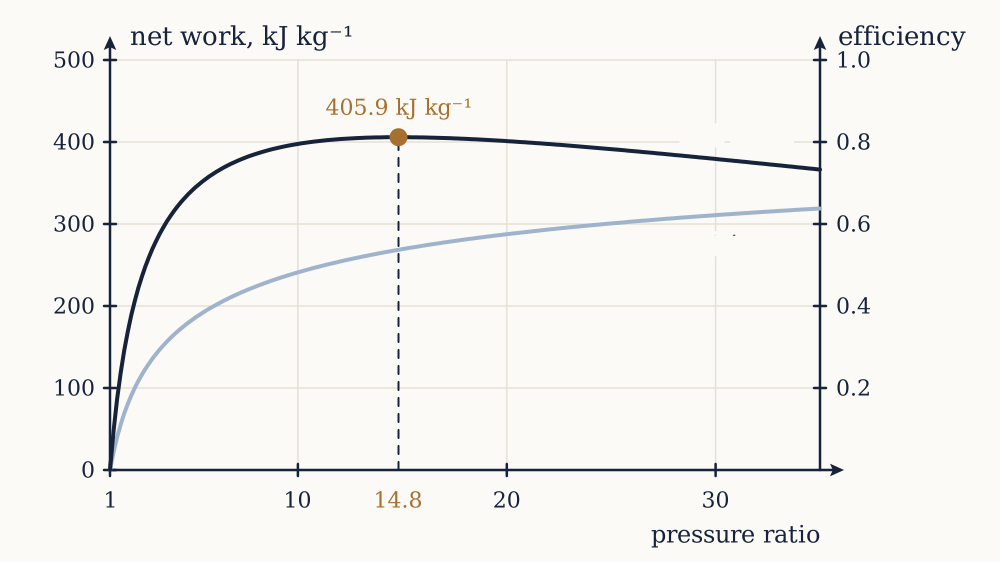
Flow work and the energy equation

A kilogram of steam entering a turbine brings its internal energy with it, and that is not the whole story, because something had to push it through the inlet.

The question the mass balance left open

Drawing a boundary around a piece of hardware and counting the mass through its ports, as the previous lesson did, says nothing about energy. To get an energy balance we need to know what each kilogram carries as it crosses, and the naive answer is wrong in an interesting way.

The naive answer is internal energy, u, the thing the First Law is written in for a closed system. A kilogram of steam at 3 MPa and 350 degrees Celsius has u=2844 kJ kg⁻¹, so surely a kilogram entering a turbine delivers 2844 kJ into the control volume. It delivers more, and the reason is mechanical rather than thermal.

Picture the inlet port with the fluid behind it. That fluid is at 3 MPa, and it is pressing on the kilogram in front of it. As the kilogram moves through the port and into the control volume, the fluid behind does work on it, and that work enters the control volume just as surely as the internal energy does. Nobody pushed anything across the boundary of a closed system, so this term has no closed-system counterpart. It is genuinely new, and it is called flow work.

The cost of the push

Compute it. Take a plug of fluid of mass m, occupying volume V=mv, being pushed through a port of area A by the pressure p immediately upstream. The plug is a cylinder of length L=V/A. The force on its rear face is pA, constant while the plug goes through, and it acts through distance L, so the work done on it is

Wflow=pAL=pAVA=pV=mpv

Per kilogram, the flow work is pv, in joules per kilogram when p is in pascals and v in m³ kg⁻¹. Notice what dropped out: the area cancelled. A narrow port needs a long plug and a wide one a short plug, and the product is the same. The push costs pv per kilogram regardless of the pipework.

The numbers are not small. For steam at 3 MPa with v=0.09056 m³ kg⁻¹, pv=3000×0.09056=271.7 kJ kg⁻¹, which is nearly ten per cent of the internal energy. At the turbine exhaust, 10 kPa with v=12.71 m³ kg⁻¹, pv=127.1 kJ kg⁻¹, still substantial despite the pressure having fallen by a factor of 300, because the volume rose by a factor of 140.

At an outlet the same argument runs with the sign flipped: the fluid leaving has to shove the fluid downstream out of its way, so it carries pv per kilogram out of the control volume. Both ports therefore contribute pv alongside u, entering at inlets and leaving at outlets.

Example. Steam at 3 MPa and 350 degrees Celsius has v=0.09056 m³ kg⁻¹ and h=3116.1 kJ kg⁻¹. Find the flow work per kilogram at that port and hence the internal energy.

Flow work is pv=3000kPa×0.09056m³ kg-1=271.7 kJ kg⁻¹, the units working because a kilopascal times a cubic metre is a kilojoule. Since h=u+pv by definition, u=3116.1-271.7=2844.4 kJ kg⁻¹, which is what the superheated table lists.

Now you. At the turbine exhaust the steam is a wet mixture at 10 kPa with v=12.71 m³ kg⁻¹ and h=2263.5 kJ kg⁻¹. Find the flow work and the internal energy.

Answer

pv=10×12.71=127.1 kJ kg⁻¹, so u=2263.5-127.1=2136.4 kJ kg⁻¹. The saturation table gives uf+xufg=191.79+0.8661×2245.4=2136.5 kJ kg⁻¹, which agrees.

Enthalpy is what flows

So the energy carried per kilogram through a port is u+pv, and that combination already has a name. It is the enthalpy,

h=u+pv

introduced in the previous course as the correct bookkeeping for a constant-pressure closed process. Here it arrives for a completely different reason and lands on the same quantity. That is worth pausing on. In the closed-system setting, enthalpy looked like an algebraic convenience, a grouping that made ΔH=Qp come out cleanly. In the open-system setting it is not a convenience at all: u+pv is literally the energy per kilogram delivered by a flowing stream, internal energy plus the work of getting it through the door. Enthalpy is the natural energy of flow, and internal energy is the natural energy of a closed box. Once that is seen, the fact that every table in this subject is written in h rather than u stops being an editorial choice.

A stream can also carry bulk kinetic energy V2/2 and potential energy gz per kilogram, so the full content of a kilogram crossing a port is

h+V22+gz

with V in m s⁻¹ and z a height above some reference level. Watch the units: h is usually tabulated in kJ kg⁻¹ while V2/2 comes out in J kg⁻¹, so one of them has to be converted, and forgetting is a factor-of-a-thousand error that is at least loud enough to notice.

The steady-flow energy equation

Now assemble the balance. For a control volume, energy accumulates at a rate equal to what comes in minus what goes out, counting heat, work and the streams. Under steady flow nothing inside accumulates, so the rate of change of the control volume's energy is zero and everything must balance:

Q˙-W˙=outm˙(h+V22+gz)-inm˙(h+V22+gz)

This is the steady-flow energy equation, and it is the single most used result in the subject. The sign convention is the one carried over from the previous course: Q˙ is positive when heat flows into the control volume, W˙ positive when work is done by it. A turbine has positive W˙, a compressor negative, and it is usually clearer to write W˙in for a compressor and keep the number positive rather than juggle minus signs.

One point about the work term deserves care. W˙ here means shaft work, electrical work, and anything else crossing the surface, but not flow work, because flow work has already been absorbed into the enthalpies. Counting it twice is a classic mistake, and the symptom is a turbine that appears to deliver an extra 271 kJ per kilogram.

For the common case of one inlet and one outlet, divide by m˙ and write everything per kilogram:

q-w=h2-h1+V22-V122+g(z2-z1)

That is the working form. Almost every device in this course is analysed by writing this line down and then deleting the terms that do not matter, which is the business of the next lesson.

How big are the velocity and height terms

Deleting terms requires knowing their size, and here the arithmetic is decisive. Kinetic energy per kilogram is V2/2, so at 45 m s⁻¹, a typical pipe velocity, it is 452/2=1013 J kg⁻¹, or 1.01 kJ kg⁻¹. Set that beside an enthalpy of 3116 kJ kg⁻¹ and it is three parts in ten thousand.

The quadratic makes the term wake up quickly. At 100 m s⁻¹ it is 5.0 kJ kg⁻¹, at 200 m s⁻¹ it is 20 kJ kg⁻¹, and at 450 m s⁻¹ it is 101 kJ kg⁻¹. The useful rule is that below about 50 m s⁻¹ the kinetic term can be dropped without thought, between 50 and 150 m s⁻¹ it should be checked against the enthalpy change rather than the enthalpy itself, and above that it must be carried. In a nozzle it is not a correction at all: it is the entire point of the device.

Potential energy is nearly always negligible in a machine. A height difference of 30 m gives gz=9.81×30=294 J kg⁻¹, about 0.29 kJ kg⁻¹. Even the 100 m from a boiler drum to a turbine floor buys under 1 kJ kg⁻¹. The exception is hydraulic machinery, where the height difference is the energy source and the enthalpy change is what is negligible: a hydroelectric station working under a 300 m head has gz=2.94 kJ kg⁻¹ and no combustion anywhere.

Example. A turbine passes 15.61 kg s⁻¹ of steam. It enters at h1=3116.1 kJ kg⁻¹ and 45 m s⁻¹ and leaves at h2=2263.5 kJ kg⁻¹ and 200 m s⁻¹, with negligible heat loss and no height change. What power does it deliver, and how much does the kinetic term matter?

With q=0 the working form gives w=(h1-h2)+(V12-V22)/2. The enthalpy drop is 3116.1-2263.5=852.6 kJ kg⁻¹. The kinetic contribution is (452-2002)/2=-18990 J kg⁻¹, that is -19.0 kJ kg⁻¹, negative because the steam leaves faster than it arrived and takes that energy away with it. So w=852.6-19.0=833.6 kJ kg⁻¹ and W˙=15.61×833.6=13010 kW, or 13.0 MW. Ignoring the velocities entirely would have given 13.3 MW, an overestimate of 2.2 per cent.

Now you. The same turbine is fitted with a smaller exhaust so the steam leaves at 260 m s⁻¹ instead, everything else unchanged. What power does it now deliver?

Answer

The kinetic term becomes (452-2602)/2=-32790 J kg⁻¹, so w=852.6-32.8=819.8 kJ kg⁻¹ and W˙=15.61×819.8=12800 kW, or 12.8 MW. Two hundred kilowatts have been thrown down the exhaust as unrecovered velocity, which is why real machines fit a diffusing exhaust hood to convert some of it back to pressure.

Reading the equation in both directions

The balance is used two ways, and it is worth being explicit about which.

Read forwards, it is a prediction. Given the inlet state, the outlet state and the flows, it says what power or heat duty the device must have. That is the mode of the example above, and of most textbook problems.

Read backwards, it is a measurement. Given the power on a shaft and the flow through a machine, it says what the outlet state must be, which is how plant instrumentation actually works: you cannot put a thermometer inside a turbine, so the exhaust state is inferred from a load reading and a flow reading. The same reading in reverse is how a device's condition is monitored over years. A turbine whose measured enthalpy drop at rated flow falls by two per cent has fouled or eroded blading, and nobody had to open it to find out.

Example. A compressor takes 0.50 kg s⁻¹ of air, raising it from 295 K to 587 K, and its casing loses 15 kW to the surroundings. Taking air as an ideal gas with cp=1.005 kJ kg⁻¹ K⁻¹ and ignoring velocities, what shaft power does it need?

The enthalpy rise per kilogram is cpΔT=1.005×(587-295)=293.5 kJ kg⁻¹, so the streams carry away 0.50×293.5=146.7 kW more than they brought in. The heat loss removes a further 15 kW. The shaft must supply both: W˙in=146.7+15=161.7 kW. Cooling a compressor does not reduce its shaft power at a fixed outlet temperature; it increases it, because the same temperature rise now has to be paid for twice.

Now you. The same compressor is run at 0.80 kg s⁻¹ with the same inlet and outlet temperatures, and its heat loss rises to 25 kW. What shaft power does it need?

Answer

W˙in=0.80×293.5+25=234.8+25=259.8 kW.

What this equation cannot tell you

Two limits should be stated before the equation is turned loose on hardware.

The first is that it is a balance, not a prediction of performance. Nothing in it says how much work a turbine will produce from a given inlet state, because the outlet state is an input, not an output. Given 3 MPa and 350 degrees Celsius at inlet and 10 kPa at exhaust, the energy equation is equally happy with an exhaust enthalpy of 2264 kJ kg⁻¹, which is a good turbine, or 3116 kJ kg⁻¹, which is a turbine that produces nothing at all and simply lets the steam through. Both conserve energy exactly. Choosing between them needs the Second Law, and that is what makes the isentropic device and its efficiency, several lessons ahead, necessary rather than decorative.

The second is that steadiness has been assumed throughout, and with it the promise that nothing inside the control volume is changing. Real plant starts, stops, trips and swings load, and a boiler drum whose level is falling is storing energy in a way this equation cannot see. Handling those is the next lesson, and the answer will turn out to explain something as everyday as why a scuba cylinder is hot to the touch after filling.

The steady-flow devices

Almost every component in a power station, a refrigerator or a jet engine is analysed by writing down the same equation and then deleting most of it.

One equation, six deletions

The previous lesson produced, for a control volume with one inlet and one outlet running steadily,

q-w=h2-h1+V22-V122+g(z2-z1)

with q and w per kilogram of fluid, heat positive inwards and work positive outwards. It has five terms and no device uses all five. What distinguishes a nozzle from a turbine is not a different physical law, it is which terms survive.

The deletions are not arbitrary, and each one is a claim about the hardware that can be checked. Saying a turbine is adiabatic is a claim that its casing loses less than about one per cent of the power passing through, which is true of a lagged machine and false of an uninsulated one. Saying a throttle has no kinetic term is a claim about the pipe diameters either side. The habit worth building is to write the full equation, then justify each deletion out loud, because the deletions are where the physics is.

Nozzles and diffusers

A nozzle is a duct shaped to raise a fluid's velocity at the expense of its pressure; a diffuser is the same device used in reverse, slowing the flow and raising the pressure. Neither has any moving part, so w=0. The fluid is inside for a few milliseconds and the surface area is small, so q0. There is no height change worth counting. Every term dies except two:

h1+V122=h2+V222

Enthalpy converts to velocity, one for one. The quantity on each side, called the stagnation enthalpy, is what a nozzle conserves.

The velocities are large by construction, so this is the one device where the kinetic term is never negligible. It is also the device where the mass balance from the earlier lesson bites hardest: since m˙=AV/v is fixed, the area must follow A=m˙v/V, and whether a duct that accelerates a fluid gets narrower or wider depends on whether v grows faster than V does. For a liquid, or for a gas below the speed of sound, V wins and the duct converges. Above the speed of sound v wins and the duct must diverge, which is why a rocket nozzle has a throat and then flares out. That result belongs to compressible flow rather than to thermodynamics, but the energy equation above is what it is built on.

Example. Air enters a nozzle at 200 degrees Celsius and 30 m s⁻¹ and leaves at 100 degrees Celsius. Taking air as an ideal gas with cp=1.005 kJ kg⁻¹ K⁻¹, what is the exit velocity?

For an ideal gas h2-h1=cp(T2-T1)=1.005×(-100)=-100.5 kJ kg⁻¹, a fall of 100500 J kg⁻¹. So V22/2=V12/2+100500=450+100500=100950 J kg⁻¹ and V2=2×100950=449 m s⁻¹. A hundred kelvin of temperature is worth four hundred and fifty metres per second, which is the trade every jet and rocket lives on.

Now you. Air enters a nozzle at 400 degrees Celsius and 20 m s⁻¹ and leaves at 250 degrees Celsius. What is the exit velocity?

Answer

cpΔT=1.005×150=150.75 kJ kg⁻¹, so V22/2=200+150750=150950 J kg⁻¹ and V2=549 m s⁻¹.

Run the same equation backwards for a diffuser. An aircraft intake takes air at 250 m s⁻¹ relative to the aeroplane and slows it to 30 m s⁻¹ before the compressor. The temperature rise is (V12-V22)/2cp=(2502-302)/(2×1005)=30.6 K, achieved with no machinery at all. At supersonic speeds this ram effect does a large part of the compression, which is why a ramjet needs no compressor and why it cannot work standing still.

Turbines

A turbine lets a fluid expand across rotating blade rows and takes work out through a shaft. The kinetic terms are small compared with the enthalpy drop, at least once the exhaust hood has been included in the control volume, and a lagged casing loses well under one per cent of the throughput as heat. So q=0, the velocity and height terms go, and

w=h1-h2

The work per kilogram is the enthalpy drop, and nothing else. A turbine passing 15.61 kg s⁻¹ of steam from h1=3116.1 to h2=2263.5 kJ kg⁻¹ delivers 15.61×852.6=13.3 MW, subject to the velocity correction computed in the previous lesson.

The equation is silent about how the enthalpy drop is achieved, which is exactly right: it holds for a steam turbine, a gas turbine, a hydraulic turbine and a wind turbine, and knows nothing about blades. What it does not tell you is how large the drop will be for a given inlet state and back pressure, and that gap is the reason the Second Law has to be brought in later.

Compressors, fans and pumps

Reverse the shaft and the same analysis gives a machine that raises pressure at the cost of work. The three names are the same device at different duties: a fan moves a lot of gas against a small pressure rise, a compressor raises gas pressure substantially, and a pump does the same to a liquid. Dropping the same terms,

win=h2-h1

with the sign taken care of by naming the work as an input. Compressors are sometimes deliberately cooled, in which case q is not zero and must be carried, as in the worked example of the previous lesson.

The interesting comparison is between a pump and a compressor working over the same pressure range, because it explains a fact that dominates the design of power stations. Water at 10 kPa has a specific volume of 0.001010 m³ kg⁻¹ and saturated steam at the same pressure has 14.67 m³ kg⁻¹, a ratio of 14500. Raising the water from 10 kPa to 3 MPa costs about 3.0 kJ kg⁻¹, which is 0.35 per cent of the 852.6 kJ kg⁻¹ the turbine delivers over the same pressure range. Compressing the vapour instead would cost of the same order as the turbine gives back. Pressurise the liquid, never the vapour: it is the whole reason the Rankine cycle exists in the form it does, and the reason a feed pump on a 600 MW station absorbs about 1.4 MW.

Throttling valves

A throttling valve is any restriction that drops pressure without any intention of extracting work: a partly open valve, an orifice plate, a porous plug, a capillary tube. There is no shaft, so w=0. The device is small and fast, so q=0. The pipes either side are usually similar, so the velocities roughly cancel, and there is no height change. Everything is gone except

h1=h2

Throttling is isenthalpic. That is a strange-looking result: pressure falls by a large factor and enthalpy does not move at all. What happens internally is that flow work is converted into internal energy by friction and turbulence, and the sum u+pv comes out unchanged even though both parts of it change a lot.

For an ideal gas, whose enthalpy depends on temperature alone, constant enthalpy means constant temperature, and throttling does nothing thermally. For a real fluid it can do a great deal. The temperature change per unit pressure drop at constant enthalpy is the Joule-Thomson coefficient, and its sign flips at a substance's inversion temperature. Nitrogen's is 621 K, so nitrogen throttled from room temperature cools, which is the basis of the Linde process for liquefying air. Hydrogen's is 202 K, so hydrogen throttled from room temperature warms, and any attempt to liquefy it by throttling alone must precool it first, a fact discovered expensively.

The dramatic case is a saturated liquid, where throttling causes flash evaporation and a large temperature drop. This is what happens in the expansion valve of every refrigerator.

Example. Saturated liquid R-134a at 800 kPa, where hf=95.47 kJ kg⁻¹ and the saturation temperature is 31.31 degrees Celsius, is throttled to 132.8 kPa, where hf=25.49 and hfg=212.91 kJ kg⁻¹ at a saturation temperature of -20 degrees Celsius. What emerges?

Enthalpy is unchanged, so the exit state has h=95.47 kJ kg⁻¹ at 132.8 kPa. Since that lies between hf=25.49 and hg=238.40, it is a wet mixture, of quality

x=h-hfhfg=95.47-25.49212.91=0.329

So a third of the liquid flashes to vapour, and the mixture sits at -20 degrees Celsius. A valve costing a few pounds has produced a 51 K temperature drop with no moving parts, no work and no heat. The evaporating third is what absorbs heat from the cold space, and the other two thirds are along for the ride.

Now you. The same saturated liquid at 800 kPa is throttled to 200 kPa instead, where hf=38.43 and hfg=206.03 kJ kg⁻¹ at -10.1 degrees Celsius. What quality results?

Answer

x=(95.47-38.43)/206.03=0.277. Less flashing, because less cooling is being asked for, and a smaller share of the flow is doing useful work in the evaporator.

Heat exchangers

A heat exchanger brings two streams into thermal contact without mixing them: a shell full of tubes, a plate stack, a coil in a tank. Draw the control surface around the whole unit and there is no shaft, no significant velocity change and, since the outside is insulated, no heat crossing the outer boundary. What is left is that whatever one stream loses, the other gains:

m˙A(hA2-hA1)=m˙B(hB1-hB2)

The heat transferred between them does not appear, because it never crossed the surface we drew: it went from one stream to the other inside it. Draw the surface around one stream only and the same heat reappears explicitly as Q˙. Both control volumes are correct, and choosing between them is choosing which question to answer.

Example. The condenser of the turbine above receives 15.61 kg s⁻¹ of steam at h=2263.5 kJ kg⁻¹ and returns it as saturated liquid at 10 kPa, where hf=191.81 kJ kg⁻¹. Cooling water enters at 18 degrees Celsius and may rise by 10 K, with c=4.18 kJ kg⁻¹ K⁻¹. What is the heat duty and how much cooling water is needed?

Per kilogram of steam, 2263.5-191.81=2071.7 kJ is rejected, so the duty is 15.61×2071.7=32340 kW, or 32.3 MW. The water side must absorb the same, so m˙w=32340/(4.18×10)=774 kg s⁻¹.

Now you. Environmental limits cut the permitted water temperature rise to 8 K. What flow is now needed?

Answer

m˙w=32340/(4.18×8)=967 kg s⁻¹, a quarter more water for the same duty.

Scale that up and the number becomes a siting constraint. A 600 MW steam plant passing 462 kg s⁻¹ rejects about 957 MW in its condenser, needing roughly 23 m³ s⁻¹ of cooling water for a 10 K rise. That is why large thermal stations sit on rivers, estuaries or coastlines, or else pay an efficiency penalty for cooling towers.

Mixing chambers, and choosing the surface

A mixing chamber is a heat exchanger with the wall removed: the streams join. There is no work and, if it is insulated, no heat, so the balance is enthalpy in equals enthalpy out,

m˙1h1+m˙2h2=m˙3h3

alongside m˙1+m˙2=m˙3 from the mass balance. Two equations, and typically two unknowns. Mixing 2.0 kg s⁻¹ of water at 80 degrees Celsius with 5.0 kg s⁻¹ at 20 degrees Celsius gives 7.0 kg s⁻¹ at (2×80+5×20)/7=37.1 degrees Celsius, taking the specific heat as constant. A domestic mixer tap is exactly this calculation. So is the open feedwater heater that will turn out to raise the efficiency of a power station by several points.

That leaves the point this lesson has been circling. The equations above are not six different results; they are one result plus six defensible sets of deletions. What actually varies between problems is where the control surface goes, and drawing it in the right place is worth more than any formula. Put it around a condenser and the heat vanishes into an internal transfer. Put it around one stream and the heat reappears. Put it around a whole power station and every internal flow disappears, leaving fuel in, air in, stack out, cooling water out and electricity out, which is the right surface for asking what the plant does and the wrong one for asking which component is at fault.

Two limits are worth naming before moving on. First, every deletion above assumed steady operation, and none of these balances survives a machine that is filling, emptying or changing load. Second, and more seriously, not one of these equations decides how well a device performs. The turbine relation w=h1-h2 is satisfied by a perfect machine and by a broken one; the compressor relation is satisfied by an efficient compressor and by a heater with an impeller in it. Energy accounting alone cannot tell them apart, and the missing ingredient is entropy.

Charging and emptying

Fill a scuba cylinder and it becomes hot enough to be uncomfortable to hold, which the steady-flow energy equation has nothing to say about, because a cylinder being filled is not steady.

The assumption that just broke

Every result so far rested on the same claim: nothing inside the control volume changes with time. That let the mass balance collapse to inflow equals outflow, and it let the energy balance drop the term describing energy accumulating inside. Both collapses are what made the analysis arithmetic.

Charging and discharging break the claim on purpose. A compressed air receiver being filled has rising mass, rising pressure and rising temperature inside it. A gas cylinder being vented has all three falling. A steam accumulator absorbing a load swing exists precisely to store and release, and a boiler drum whose level moves during a load change is storing water and energy in a way no steady balance can see.

These are not exotic cases. Every plant spends its riskiest hours starting up and shutting down, safety relief devices operate only in transients, and a large fraction of pressure-vessel incidents happen during filling or emptying. The analysis needed is not much harder, but it has one extra term and one new modelling decision.

The transient balance

Keep the same control volume and stop deleting the accumulation terms. Conservation of mass, integrated over a process from state 1 to state 2, gives

m2-m1=min-mout

and conservation of energy, with the energy inside the control volume written as mu since it is not moving anywhere,

Q-W=m2u2-m1u1+mouthout-minhin

Both are exact. Notice which energy appears where: the contents of the control volume are counted with u, because nothing is pushing them anywhere, while everything crossing a port is counted with h, because it had to be pushed. That distinction, arbitrary-looking when enthalpy was first introduced, is doing real work here, and getting it backwards is the standard way to produce a wrong answer that looks reasonable.

The new modelling decision is what value of h to use at a port, since the state at the port can change during the process. The uniform-flow model assumes it does not: the fluid crossing each port has one fixed state for the whole process, and the contents of the control volume, while changing in time, are uniform in space at any instant. For a bottle filled from a large line at fixed pressure and temperature this is very good. For a bottle discharging, the fluid leaving is at the instantaneous state inside, which is changing, and the model is worse. That case is handled below.

Filling an empty bottle

Take the simplest possible case and let it produce a result nobody expects.

A rigid, insulated, evacuated bottle is connected to a large line carrying air at fixed pressure and temperature, and the valve is opened until the pressure inside equals the line pressure. The bottle is rigid so W=0, insulated so Q=0, initially evacuated so m1=0, and nothing leaves. The energy balance reduces to a single line:

m2u2=minhline

and the mass balance says min=m2. Cancel it:

u2=hline

The final internal energy inside the bottle equals the enthalpy of the fluid in the line. That is the whole result, and it is remarkable because there is no heating of any kind: nothing burned, nothing rubbed, no work crossed the boundary. What happened is that the line did flow work pv per kilogram to shove the air through the valve, and that work had nowhere to go but into the internal energy of the air now sitting inside.

For an ideal gas with constant specific heats, u2=cvT2 and hline=cpTline, so

T2=cpcvTline=kTline

The gas in the bottle ends up hotter than the supply by the factor k, which for air is 1.400. Air from a line at 300 K fills a bottle at 420 K, a rise of 120 K, independent of the pressure, the volume and the size of the valve. Anyone who has filled a diving cylinder or a car tyre from a compressor has felt this, and much of what they felt was this rather than the compressor's own heat.

Example. A rigid, insulated, evacuated 0.500 m³ vessel is filled from a line carrying air at 700 kPa and 300 K until the pressure inside reaches 700 kPa. Find the final temperature and the mass admitted, taking R=0.287 kJ kg⁻¹ K⁻¹ and k=1.400.

The temperature follows immediately: T2=kTline=1.400×300=420 K, or 147 degrees Celsius. The mass then comes from the ideal gas law at the final state, m2=p2V/RT2=(700)(0.500)/(0.287×420)=2.90 kg. Had the filling somehow been isothermal at 300 K, the bottle would have held (700)(0.500)/(0.287×300)=4.07 kg, forty per cent more. The vessel will in fact reach that mass only if it is refilled after cooling.

Now you. A rigid, insulated, evacuated 0.300 m³ vessel is filled from a line at 1.20 MPa and 290 K. Find the final temperature and the mass admitted.

Answer

T2=1.400×290=406 K, and m2=(1200)(0.300)/(0.287×406)=3.09 kg.

The corollary matters commercially. Let the filled bottle sit until it returns to 300 K and its pressure falls to 700×300/420=500 kPa, since the mass and volume are fixed. A cylinder charged to its rated pressure while hot is not full once it cools, which is why a properly filled cylinder is either filled slowly, filled in a water bath, or topped up afterwards.

Filling a bottle that is not empty

Drop the requirement that the vessel starts empty and the algebra grows one term. With m1 already inside at temperature T1, the energy balance is m2u2-m1u1=(m2-m1)hline, and for an ideal gas that reads

cv(m2T2-m1T1)=(m2-m1)cpTline

The unknowns are m2 and T2, and the second equation needed is the ideal gas law at the final state, m2T2=p2V/R, whose right-hand side is entirely known. Substituting turns the pair into one linear equation in m2.

Example. The same rigid insulated 0.500 m³ vessel already contains air at 100 kPa and 300 K. It is filled from the same line at 700 kPa and 300 K until the pressure inside reaches 700 kPa. Find the final temperature and mass. Use cv=0.718 and cp=1.005 kJ kg⁻¹ K⁻¹.

The initial mass is m1=(100)(0.500)/(0.287×300)=0.5807 kg. The product m2T2 is fixed by the final pressure: m2T2=p2V/R=(700)(0.500)/0.287=1219.5 kg K. Put both into the balance:

0.718×1219.5-0.5807×0.718×300=(m2-0.5807)(1.005)(300)

The left side is 875.6-125.1=750.5 kJ. The right side is 301.5m2-175.1, so 301.5m2=925.6 and m2=3.070 kg. Then T2=1219.5/3.070=397 K. The air already present, which does not have to be pushed in and so brings no flow work, drags the final temperature below the 420 K of the empty case.

Now you. The same vessel starts at 200 kPa and 300 K instead. Find m2 and T2.

Answer

m1=(200)(0.500)/(0.287×300)=1.161 kg. The balance becomes 875.6-250.2=301.5m2-350.2, so 301.5m2=975.6, giving m2=3.236 kg and T2=1219.5/3.236=377 K.

Blowing a vessel down

Discharge is the harder direction, because the fluid leaving is at the state inside the vessel, and that state is changing throughout. The uniform-flow assumption of a fixed port state is simply false.

There is a clean way through it for the commonest case. Follow the gas that remains in the vessel at the end. It never crossed the boundary, so it is a closed system. It expanded, because the gas that left made room for it. If the vessel is insulated and the expansion is slow enough to stay near equilibrium, that remaining gas has undergone a reversible adiabatic expansion, and for an ideal gas the isentropic relation applies directly:

T2T1=(p2p1)(k-1)/k

No transient balance was needed. The trick is choosing the system: the residual gas, not the vessel's contents as a whole.

Example. The 0.500 m³ vessel above, holding air at 700 kPa and 420 K, is vented to atmosphere at 100 kPa through a valve. Taking the process as adiabatic and the remaining gas as expanding reversibly, find the final temperature and the mass left.

The pressure ratio is 100/700 and the exponent is (k-1)/k=0.2857, so T2=420×(1/7)0.2857=420×0.5735=241 K, which is -32 degrees Celsius. The mass left is m2=(100)(0.500)/(0.287×241)=0.723 kg, against 2.90 kg initially, so three quarters of the air has gone.

Now you. The same vessel is vented only to 300 kPa. Find the final temperature and the mass remaining.

Answer

T2=420×(3/7)0.2857=420×0.7850=330 K, or 57 degrees Celsius, and m2=(300)(0.500)/(0.287×330)=1.58 kg, so 45 per cent has escaped.

That -32 degrees Celsius is visible: vent a gas cylinder quickly and frost forms on it, and the valve can ice up hard enough to jam. It is also a hazard, since carbon steel loses toughness as it cools and a vessel designed for ambient temperature may be blown down into a range where it is brittle. Depressurisation rates in process plant are limited for exactly this reason.

Where the model earns its keep, and where it fails

The uniform-flow model is a genuine approximation and it is worth being specific about what it costs.

It assumes the contents are uniform at every instant. In a bottle being filled fast, the incoming jet is nothing like uniform, and the gas near the inlet is much hotter than the gas at the far end until mixing catches up. The final equilibrium temperature is still right, because the balance only used end states, but any statement about what the gas was doing halfway through is not.

It assumes the process is slow enough that the pressure inside is meaningful. Fast discharge through a small orifice is choked, the flow is sonic at the throat, and the gas inside is not in equilibrium with itself. The isentropic blowdown result then overestimates the cooling, because heat leaks in from the vessel walls, which have far more heat capacity than the gas and act as a reservoir. Real blowdown of a steel cylinder is nearer isothermal than isentropic for slow vents and nearer isentropic for fast ones, and both bounds are worth computing to bracket the answer.

It assumes, in the filling result, that the gas is ideal with constant specific heats. For air at these pressures that is fine. For a bottle being charged to 200 bar it is not, and the compressibility factor has to come back.

None of these transients said anything about how much of the process was avoidable. Filling a bottle from a line at 300 K and ending at 420 K wastes something: that heat leaks away and the cylinder ends up holding less gas than it could. The energy balance is perfectly happy and reports no loss at all, because energy was conserved exactly. To say that the process was wasteful, and by how much, needs a quantity that increases when something irreversible happens, and applying that quantity to control volumes is the next lesson.

Isentropic efficiency

Given steam entering a turbine at 3 MPa and 350 degrees Celsius and leaving at 10 kPa, the energy balance is equally content with a machine that produces 980 kJ per kilogram and one that produces nothing at all.

The gap the energy balance leaves

The steady-flow energy equation says w=h1-h2 for an adiabatic turbine, and that is a true statement about any turbine. It is also a statement with two unknowns in it. Nothing in the First Law fixes h2, so nothing in the First Law fixes the work. Feed the equation an exhaust enthalpy of 2136 kJ kg⁻¹ and the turbine is excellent; feed it 3116 kJ kg⁻¹ and the steam has passed through unchanged, producing nothing, while conserving energy perfectly.

The same hole appears everywhere. A compressor that raises air from 100 to 800 kPa may deliver it at 534 K or at 700 K, and the energy balance simply reports a larger work input in the second case without complaint. A nozzle may reach 449 m s⁻¹ or 400 m s⁻¹ from the same inlet state. In each case the missing statement is not about energy but about direction, and the previous course established what supplies it.

The entropy balance for a control volume

Entropy is not conserved. It is transferred with heat, carried by mass, and generated by irreversibility, and the balance says so term by term. For a control volume,

dScvdt=Q˙Tb+inm˙s-outm˙s+S˙gen

where Tb is the temperature of the boundary where the heat crosses, and S˙gen0 always, equalling zero only for a reversible process. The second and third terms are new relative to the closed-system version, and they are simple: a kilogram crossing a port takes its entropy with it, exactly as it takes its enthalpy.

Under steady operation the left side vanishes, and for one inlet and one outlet the balance rearranges to

S˙gen=m˙(s2-s1)-Q˙Tb0

Now make the device adiabatic, which as the earlier lesson argued is a good description of a turbine, a compressor, a nozzle or a valve. The heat term goes and what is left is stark:

s2s1

An adiabatic steady-flow device cannot lower the entropy of the fluid passing through it. Not "usually does not": cannot. Every real one raises it, and the amount by which it does is S˙gen/m˙, a direct measure of how badly the device is behaving.

The ideal device is the isentropic one

The inequality has a boundary, and the boundary is the benchmark we were missing. The best conceivable adiabatic device is the one that generates no entropy at all, so it operates at s2=s1 and is called isentropic. Isentropic means adiabatic and reversible together, and neither half alone is enough: a throttling valve is adiabatic and hopeless.

The isentropic device is not achievable, and that does not weaken it. It is a fixed, computable target defined by the inlet state and the exit pressure alone, which is exactly what a benchmark has to be. Given 3 MPa and 350 degrees Celsius at inlet and 10 kPa at exhaust, the isentropic exit state is fully determined: s2=s1=6.7450 kJ kg⁻¹ K⁻¹, which at 10 kPa where sf=0.6492 and sfg=7.4996 gives a quality

x2s=6.7450-0.64927.4996=0.8128

and hence h2s=191.81+0.8128×2392.1=2136.2 kJ kg⁻¹. The ideal work is 3116.1-2136.2=980.0 kJ kg⁻¹, and no adiabatic turbine between those states can beat it.

For an ideal gas with constant specific heats the isentropic exit state comes from a formula rather than a table. Starting from ds=cpdT/T-Rdp/p and setting ds=0,

T2T1=(p2p1)(k-1)/k

with k=cp/cv, which for air is 1.400 and gives an exponent of 0.2857. This one relation carries most of the gas turbine work later in the course.

Reversible work, and why pumping liquid is cheap

Before scoring real machines, one result explains a fact that has been asserted twice already. For a reversible steady-flow process, the work per kilogram is

wrev=-12vdp

ignoring velocity and height changes. The derivation is two lines. The property relation Tds=dh-vdp holds for any substance between any two equilibrium states. For a reversible process δq=Tds, and the energy equation in differential form is δq-δw=dh. Substitute: δw=Tds-dh=Tds-(Tds+vdp)=-vdp. Integrate.

Read it as an instruction. The work of a steady-flow machine is set by the specific volume of whatever is being pushed against the pressure change. To spend little, arrange for v to be small, which means compress liquids and expand vapours, never the reverse.

The numbers are brutal. Water at 10 kPa has v=0.001010 m³ kg⁻¹ and is nearly incompressible, so the integral is just v(p2-p1). Raising it to 15 MPa costs 0.001010×14990=15.1 kJ kg⁻¹. Saturated steam at the same 10 kPa has v=14.67 m³ kg⁻¹, fourteen thousand times larger, and compressing it over the same range would cost of the order of the entire output of the turbine. This is why every vapour power cycle condenses its working fluid completely before raising its pressure, and it is the single most consequential line in this course.

Example. A boiler feed pump raises water from saturated liquid at 10 kPa, where v=0.001010 m³ kg⁻¹, to 15 MPa. Its isentropic efficiency is 0.85. Find the ideal and actual work per kilogram, and the power required at 462 kg s⁻¹.

Treating the water as incompressible, ws=v(p2-p1)=0.001010×(15000-10)=15.14 kJ kg⁻¹. A pump's efficiency is ideal work over actual, since work is being paid for, so wa=15.14/0.85=17.81 kJ kg⁻¹. The power is 462×17.81=8230 kW, or 8.2 MW, out of a station producing several hundred.

Now you. A smaller plant pumps the same water from 10 kPa to 5 MPa with a pump of isentropic efficiency 0.80. Find the ideal and actual work per kilogram.

Answer

ws=0.001010×4990=5.04 kJ kg⁻¹ and wa=5.04/0.80=6.30 kJ kg⁻¹.

Turbine isentropic efficiency

Now the definition. For a turbine, work is the product, so the efficiency is what you got over what you could have got, both taken between the same inlet state and the same exit pressure:

ηT=waws=h1-h2ah1-h2s

Large steam turbines reach 0.88 to 0.92, gas turbines 0.85 to 0.90, small machines much less. The definition has a subtlety worth stating: h2a and h2s are at the same pressure but not the same state. The real turbine ends at a higher entropy, and therefore at a higher enthalpy, than the ideal one.

Example. The turbine above, taking steam at 3 MPa and 350 degrees Celsius and exhausting to 10 kPa, has ηT=0.87. Find the actual work and the actual exit state.

The ideal work was computed above as 980.0 kJ kg⁻¹, so the actual work is 0.87×980.0=852.6 kJ kg⁻¹ and the actual exit enthalpy is h2a=3116.1-852.6=2263.5 kJ kg⁻¹. That is still inside the dome at 10 kPa, at a quality of (2263.5-191.81)/2392.1=0.866, against 0.813 for the ideal machine. The real turbine exhausts drier than the ideal one, because the losses reappear as internal energy in the fluid and re-evaporate some of the moisture. The entropy generated is s2a-s1=7.144-6.745=0.399 kJ kg⁻¹ K⁻¹, and a later lesson will convert that number into wasted joules.

Now you. A worn machine on the same duty manages ηT=0.80. Find its actual work, exit enthalpy and exit quality.

Answer

wa=0.80×980.0=784.0 kJ kg⁻¹, so h2a=3116.1-784.0=2332.1 kJ kg⁻¹ and x=(2332.1-191.81)/2392.1=0.895.

Compressors, pumps and nozzles

For a device that consumes work the ratio is inverted, so that the efficiency is again a number below one:

ηC=wswa=h2s-h1h2a-h1

Typical values run from 0.75 for a small machine to 0.90 for a large axial compressor. Pumps are defined identically and reach 0.70 to 0.90.

Example. A compressor takes air at 100 kPa and 295 K and delivers it at 800 kPa. Its isentropic efficiency is 0.82. With cp=1.005 kJ kg⁻¹ K⁻¹ and k=1.400, find the ideal work, the actual work and the delivery temperature.

The isentropic exit temperature is T2s=295×80.2857=295×1.8115=534.4 K, so ws=cp(T2s-T1)=1.005×239.4=240.6 kJ kg⁻¹. The actual work is wa=240.6/0.82=293.4 kJ kg⁻¹, and since the air really does absorb all of it, T2a=295+293.4/1.005=587 K, or 314 degrees Celsius. Fifty-two kelvin of that is pure inefficiency, and it has to be got rid of downstream.

Now you. A cheaper machine on the same duty has ηC=0.75. Find its actual work and delivery temperature.

Answer

wa=240.6/0.75=320.8 kJ kg⁻¹ and T2a=295+320.8/1.005=614 K, which is 341 degrees Celsius.

A nozzle produces neither work nor heat, so its efficiency is written in kinetic energy: ηN=V2a2/V2s2, the ratio of actual to ideal exit kinetic energy. Well-designed nozzles are extremely good, 0.90 to 0.97, because the flow is accelerating and accelerating flows do not separate from walls. The air nozzle of an earlier lesson, ideally reaching 449 m s⁻¹, manages 4490.95=438 m s⁻¹ at ηN=0.95.

Diffusers are the mirror image and are much worse, often 0.70 to 0.85, because there the flow is decelerating against a rising pressure and will separate at the smallest excuse. Anyone who has designed a duct knows that expansions are hard and contractions are easy, and this is the thermodynamic statement of it.

What the benchmark does not say

Three honest limits, because the number is used more casually than it deserves.

First, isentropic efficiencies are not comparable across devices. A turbine at 0.87 and a compressor at 0.87 generate different amounts of entropy on the same duty, because the two definitions divide by different things. Comparing them properly needs a common currency, which is what the exergy lesson supplies.

Second, a multistage turbine's overall isentropic efficiency exceeds the efficiency of its individual stages, which sounds impossible and is not. Each stage's losses reheat the fluid, and the reheated fluid arriving at the next stage has slightly more enthalpy available to drop, since the constant-pressure lines on an enthalpy-entropy diagram diverge as entropy rises. Some of each stage's loss is therefore recovered downstream. The effect, called the reheat factor, is worth two to four points on a large machine, and it means a stage efficiency quoted as an overall one is being flattered.

Third, the benchmark is silent on devices whose ideal work is zero. A throttling valve has ws=0 and wa=0, so the definition gives nothing at all, yet the valve is thoroughly irreversible: the R-134a valve of an earlier lesson generates 0.0174 kJ kg⁻¹ K⁻¹ every time a kilogram goes through it. Isentropic efficiency measures how well a device does the job it was built for. It cannot notice a device whose job is to waste something.

With efficiencies for the individual machines in hand, the pieces can finally be chained together: the exhaust of one device becomes the inlet of the next, and the last one feeds back into the first. That closed chain is a cycle, and it is where this course starts producing power.

Cycles and the mean temperature

A turbine on its own is not a power station, because after one pass the working fluid has been used up and thrown away.

Closing the loop

Each device analysed so far takes a fluid from one state to another and stops. Expand steam through a turbine and you have low-pressure wet steam and a shaft turning; expand it again and nothing happens, because it is already at the exhaust pressure. To keep producing work indefinitely the fluid has to be brought back to its starting state and sent round again, and the sequence of processes that does that is a cycle.

That is not merely a convenience about not wasting water. A cycle is what makes continuous power possible from a finite quantity of working fluid, and closing the loop imposes conditions of its own that shape every real plant. The fluid leaves the turbine at low pressure, and something has to raise it again. Raising a vapour's pressure is ruinously expensive, as the reversible work integral showed, so the vapour is condensed first and a pump does the job instead. That single decision determines the layout of every steam plant on earth.

For a cycle, the working fluid returns to its initial state, so every property returns with it: du=0, dh=0, ds=0. Applying the energy balance around the whole loop, with the enthalpy change summing to zero,

wnet=qin-qout

The net work equals the net heat, per kilogram of fluid circulated. Nothing is stored anywhere.

Two numbers that describe any cycle

The first is the thermal efficiency, work delivered over heat paid for:

ηth=wnetqin=1-qoutqin

The second is the back work ratio, the fraction of the gross work output that the cycle has to feed back into its own compression:

bwr=wcompressionwexpansion

Efficiency gets all the attention and back work ratio decides whether a machine is buildable. A cycle with a back work ratio of 0.9 delivers a tenth of its gross work to the outside world, so a two per cent slip in either machine's efficiency wipes out a fifth of the output. It is also why gas turbines could not be built until compressor design improved: the concept is Victorian, the hardware is not.

Example. A steam plant supplies 2921 kJ of heat and rejects 1944 kJ per kilogram of steam. Its turbine delivers 980.0 kJ kg⁻¹ and its feed pump absorbs 3.02 kJ kg⁻¹. Find the net work, the thermal efficiency and the back work ratio.

The net work is 2921-1944=977 kJ kg⁻¹, which also equals 980.0-3.02=977.0 kJ kg⁻¹, and the two routes agreeing is the check that the cycle balances. The efficiency is 977/2921=0.334. The back work ratio is 3.02/980.0=0.0031, three parts in a thousand, which is the enormous structural advantage of pumping a liquid.

Now you. A gas turbine's compressor absorbs 311.8 kJ kg⁻¹ and its turbine delivers 715.3 kJ kg⁻¹, with 793.8 kJ kg⁻¹ of heat supplied. Find the net work, the efficiency and the back work ratio.

Answer

wnet=715.3-311.8=403.5 kJ kg⁻¹, ηth=403.5/793.8=0.508, and the back work ratio is 311.8/715.3=0.436. The efficiency is far better than the steam plant's and the back work ratio is a hundred and forty times worse.

The bound, and the size of the gap

The previous course established the Carnot limit: no cycle exchanging heat with reservoirs at TH and TL can beat 1-TL/TH. A steam plant with metal at 600 degrees Celsius rejecting to a condenser at 45.81 degrees Celsius has a bound of 1-318.96/873.15=0.635. Real plants of that description reach about 0.45.

The gap is not one thing. Some of it is component inefficiency, the turbines and pumps of the previous lesson falling short of isentropic. Some is heat transfer across finite temperature differences, in the boiler, in the condenser and in every feedwater heater. But a large part of it is neither, and it survives even in a cycle whose every component is perfect. Understanding that part requires a sharper statement of the limit than "Carnot".

The mean temperature of heat addition

Here is the sharpening, and it is exact rather than approximate.

Consider any cycle whose heat rejection happens at a single constant temperature TL. That is not a contrived case: a steam plant condenses at constant pressure inside the saturation dome, and constant pressure inside the dome means constant temperature. Over the rejection process, qout=Tds=TLΔs, where Δs is the entropy change of the fluid across the condenser.

Heat addition is not at a single temperature: the water enters the boiler cold, warms, boils, and superheats, so T climbs throughout. But the integral is still an integral, so define a mean temperature of heat addition by

TH=qinΔs

which is nothing more than the average of T weighted by entropy change. Since the cycle is closed, the entropy change across the boiler equals the entropy change across the condenser in magnitude, and the same Δs appears in both expressions. Divide:

ηth=1-qoutqin=1-TLΔsTHΔs=1-TLTH

A cycle with reversible components has exactly Carnot's efficiency, evaluated not at its peak temperature but at the mean temperature at which it actually takes heat in. That is the sharpening. The Carnot bound compares against the hottest metal in the plant, which is irrelevant if only a tenth of the heat goes in there.

Test it on real numbers. A steam cycle taking water from saturated liquid at 10 kPa to steam at 3 MPa and 350 degrees Celsius has qin=2921 kJ kg⁻¹ and Δs=6.7450-0.6492=6.0958 kJ kg⁻¹ K⁻¹. So TH=2921/6.0958=479.2 K, which is 206 degrees Celsius, and ηth=1-318.96/479.2=0.334. That is precisely the efficiency computed above from enthalpies, by a route that never mentioned entropy.

The lesson in the number is that 479 K is a long way below the 623 K of the superheated steam. The cycle spends a great deal of its heat input warming subcooled water from 46 to 234 degrees Celsius, and that heat goes in at low temperature and drags the mean down. Every improvement in the next lessons is an attack on this one number.

Example. A cycle takes heat at a mean temperature of 479 K and rejects at 319 K. What is the best efficiency it can have, and how does raising the superheat to 600 degrees Celsius, which lifts qin to 3488 kJ kg⁻¹ and Δs to 6.8593 kJ kg⁻¹ K⁻¹, change it?

The first is 1-319/479=0.334. For the second, TH=3488/6.8593=508.5 K, so ηth=1-318.96/508.5=0.373. Two hundred and fifty degrees of extra superheat moved the mean temperature by only 29 K, because superheating adds heat at high temperature but also adds a lot of entropy.

Now you. Raising the boiler pressure to 15 MPa at 600 degrees Celsius gives qin=3376 kJ kg⁻¹ and Δs=6.0304 kJ kg⁻¹ K⁻¹, still rejecting at 319 K. What are the mean temperature and the efficiency?

Answer

TH=3376/6.0304=560 K, so ηth=1-318.96/560=0.430. Pressure is a more effective lever than superheat, because raising the pressure raises the temperature at which the boiling itself happens.

Why nobody builds a Carnot cycle

If the Carnot cycle is the best possible, an obvious question is why every power station is not one. The answer is entirely practical, and it is worth going through because each objection explains a feature of the cycle that gets built instead.

Take the Carnot cycle executed with steam entirely inside the saturation dome, where isothermal heat transfer is automatic: boil at TH, expand isentropically, condense partially at TL, compress isentropically back to saturated liquid. Four objections, in order of severity.

The heat addition is isothermal, so it must happen inside the dome, which caps the top temperature at water's critical temperature of 373.95 degrees Celsius. Even at that cap the bound is only 0.51, and worse, the latent heat vanishes as the critical point is approached, so a cycle running near it circulates enormous quantities of water for very little heat. The metallurgical limit of a modern boiler is well above 600 degrees Celsius, and a cycle that cannot use it is throwing away its best asset.

The isentropic expansion runs from saturated vapour down to TL, ending deep in the wet region. Boiling at 3 MPa, where sg=6.1856 kJ kg⁻¹ K⁻¹, the exhaust quality at 10 kPa is (6.1856-0.6492)/7.4996=0.738, and pushing the boiling pressure to 15 MPa to chase efficiency makes it 0.622. A third of the mass arriving at the last blade row as liquid is not a thermodynamic inconvenience, it is destruction: droplets travelling at hundreds of metres per second erode blade leading edges, and practice limits the exhaust moisture to about 10 per cent.

The compression stage is worse. It takes a two-phase mixture and compresses it isentropically back to saturated liquid, and no machine exists that handles a mixture of liquid and vapour at high pressure ratio. Pumps cavitate on vapour and compressors are destroyed by liquid.

Finally, the partial condensation must be stopped at exactly the quality that makes the subsequent isentropic compression land on the saturated liquid line. Controlling a condenser to a precise intermediate quality is not something a plant operator can do.

The gas version fares no better. A Carnot cycle in a gas needs isothermal compression and isothermal expansion, meaning heat transfer at a vanishing temperature difference and therefore infinite heat exchanger area, and the isentropic legs between 300 K and 1400 K alone demand a pressure ratio of (1400/300)3.5=220. The enclosed area on the pressure-volume diagram is small compared with the swept volume, so the machine is enormous for the power it makes.

The repair

Every objection points the same way, and the fixes are all corrections to the Carnot cycle rather than replacements for it.

Condense the vapour completely to saturated liquid rather than partially, which removes the impossible two-phase compressor and replaces it with a pump. That costs a little, because heat must then be added to warm subcooled liquid at low temperature, dragging the mean temperature down. It is worth it a hundred times over: the back work ratio falls from a substantial number to 0.003.

Add heat at constant pressure rather than constant temperature, so that the cycle may leave the dome and superheat as far as the metallurgy allows. That gives up the exact isothermal ideal in exchange for a much higher peak temperature, and moves the exhaust away from the wet region.

What is left after those two changes is the Rankine cycle: pump, boiler, turbine, condenser. It is not the most efficient cycle imaginable and it is the one that can be built, and it generates the large majority of the world's electricity, whether the heat comes from coal, gas, uranium or concentrated sunlight. Analysing one completely, with real steam properties and real component efficiencies, is the next lesson.

The Rankine cycle

Most of the world's electricity is produced by boiling water, expanding the steam through a turbine, condensing it and pumping it back, and the cycle that describes this has four processes and no spare parts.

Four devices, four processes

The layout comes straight out of the repairs made to the Carnot cycle in the previous lesson. Name the states going round the loop and each device is one of the steady-flow machines already analysed.

State 1 is saturated liquid leaving the condenser, at the lowest pressure in the plant. The feed pump raises it to boiler pressure, ideally isentropically, reaching state 2: compressed liquid, still cold. The boiler adds heat at constant pressure, warming the water to its saturation temperature, boiling it, and superheating the vapour to state 3. The turbine expands it, ideally isentropically, to the condenser pressure at state 4. The condenser rejects heat at constant pressure and temperature, returning the fluid to saturated liquid at state 1.

The ideal Rankine cycle is this loop with an isentropic pump, an isentropic turbine, and no pressure drop anywhere. It is not the Carnot cycle and does not pretend to be. Heat is added at constant pressure rather than constant temperature, so the process is externally irreversible against a hot source, and the cycle's efficiency is Carnot's evaluated at the mean temperature of heat addition rather than the peak.

Each device is analysed with the steady-flow energy equation and no velocity or height terms:

wpump=h2-h1=v1(p2-p1),qin=h3-h2,wturb=h3-h4,qout=h4-h1

The pump form uses the incompressibility of liquid water, which is accurate to better than a per cent and avoids needing a compressed-liquid table.

A complete ideal cycle

Take a plant with boiler conditions of 3 MPa and 350 degrees Celsius and a condenser at 10 kPa. The saturation table at 10 kPa gives Tsat=45.81 degrees Celsius, vf=0.001010 m³ kg⁻¹, hf=191.81 kJ kg⁻¹, hfg=2392.1 kJ kg⁻¹, sf=0.6492 and sfg=7.4996 kJ kg⁻¹ K⁻¹. The superheated table at 3 MPa and 350 degrees Celsius gives h3=3116.1 kJ kg⁻¹ and s3=6.7450 kJ kg⁻¹ K⁻¹.

Work round the loop. At state 1, h1=191.81 kJ kg⁻¹. The pump work is v1(p2-p1)=0.001010×(3000-10)=3.02 kJ kg⁻¹, so h2=194.83 kJ kg⁻¹. The boiler supplies qin=3116.1-194.83=2921.3 kJ kg⁻¹.

The turbine is isentropic, so s4=s3=6.7450 kJ kg⁻¹ K⁻¹. At 10 kPa that entropy is below sg=8.1488, so the exhaust is wet, with quality

x4=6.7450-0.64927.4996=0.8128

and h4=191.81+0.8128×2392.1=2136.2 kJ kg⁻¹. The turbine therefore delivers wturb=3116.1-2136.2=980.0 kJ kg⁻¹, and the condenser rejects qout=2136.2-191.81=1944.3 kJ kg⁻¹.

Net work is 980.0-3.02=977.0 kJ kg⁻¹, which must and does equal qin-qout=2921.3-1944.3. The thermal efficiency is

ηth=977.02921.3=0.334

and the back work ratio is 3.02/980.0=0.0031.

Example. The condenser of that plant is fouled and its pressure rises from 10 kPa to 20 kPa, where vf=0.001017, hf=251.42, hfg=2357.5, sf=0.8320 and sfg=7.0752. Boiler conditions are unchanged. What happens to the efficiency?

The pump work becomes 0.001017×2980=3.03 kJ kg⁻¹ and h2=254.45 kJ kg⁻¹, so qin=3116.1-254.45=2861.7 kJ kg⁻¹. The exhaust quality is (6.7450-0.8320)/7.0752=0.8357, giving h4=251.42+0.8357×2357.5=2221.7 kJ kg⁻¹ and turbine work 894.4 kJ kg⁻¹. Net work is 891.4 kJ kg⁻¹ and ηth=891.4/2861.7=0.311.

Ten kilopascals of condenser pressure, a change of one tenth of an atmosphere at the coldest point in the plant, has cost 2.3 efficiency points, about seven per cent of the output. This is why condenser vacuum is watched obsessively, and why air in-leakage is a serious fault rather than a nuisance.

Now you. Suppose instead the plant is built on a hot river and the condenser must run at 15 kPa, where vf=0.001014, hf=225.94, hfg=2372.3, sf=0.7549 and sfg=7.2522. Find the efficiency.

Answer

wp=0.001014×2985=3.03 kJ kg⁻¹ so h2=228.97 and qin=2887.1 kJ kg⁻¹. The quality is (6.7450-0.7549)/7.2522=0.8260, giving h4=225.94+0.8260×2372.3=2185.4 kJ kg⁻¹ and wturb=930.7 kJ kg⁻¹. Net work is 927.7 kJ kg⁻¹ and ηth=927.7/2887.1=0.321, between the other two as expected.

Where the heat actually goes in

The boiler duty is one number in the efficiency calculation and three physically distinct jobs, and separating them explains the whole shape of the cycle.

StageTemperature rangeHeat, kJ kg⁻¹Share
Warming liquid to saturation46 to 234 °C812.927.8%
Boiling at 3 MPa234 °C1794.961.5%
Superheating234 to 350 °C312.910.7%

Nearly twenty-eight per cent of the heat goes into warming subcooled water between 46 and 234 degrees Celsius, all of it at temperatures far below the peak. That is what holds the mean temperature of heat addition down to 479 K when the steam leaves at 623 K, and it is the target of the regeneration scheme in the next lesson. The boiling, at a single temperature of 234 degrees Celsius, is where most of the heat goes, which is why raising the boiler pressure and therefore the boiling temperature is the strongest lever available. The superheat, despite adding the highest-temperature heat in the cycle, is only a tenth of the total.

Real components

Replace the two ideal machines with real ones. A turbine of isentropic efficiency 0.87 and a pump of 0.85 change the numbers as follows, with the isentropic values as the reference.

The pump now absorbs 3.02/0.85=3.55 kJ kg⁻¹, so h2=195.36 kJ kg⁻¹ and qin=3116.1-195.36=2920.7 kJ kg⁻¹, barely changed. The turbine delivers 0.87×980.0=852.6 kJ kg⁻¹, so h4=3116.1-852.6=2263.5 kJ kg⁻¹ at a quality of 0.866, and the condenser must now reject 2263.5-191.81=2071.7 kJ kg⁻¹. Net work is 852.6-3.55=849.0 kJ kg⁻¹ and

ηth=849.02920.7=0.291

Thirteen per cent of the ideal cycle's output has gone, essentially all of it in the turbine. Notice where it reappears: the condenser duty has risen from 1944 to 2072 kJ kg⁻¹. Energy is conserved, so work not taken by the shaft leaves through the cooling water instead.

Example. A plant with the same boiler and condenser conditions has a better turbine, ηT=0.90, and a worse pump, ηP=0.80. Find the net work and thermal efficiency.

The turbine gives 0.90×980.0=882.0 kJ kg⁻¹ and the pump absorbs 3.02/0.80=3.77 kJ kg⁻¹, so h2=195.58 and qin=2920.5 kJ kg⁻¹. Net work is 882.0-3.77=878.2 kJ kg⁻¹ and ηth=878.2/2920.5=0.301. Three points of turbine efficiency bought one point of cycle efficiency, and the pump's five-point loss cost nothing measurable, which is the back work ratio speaking.

Now you. An old machine on the same duty has ηT=0.78 and ηP=0.75. Find the net work and efficiency.

Answer

Turbine work is 0.78×980.0=764.4 kJ kg⁻¹ and pump work is 3.02/0.75=4.03 kJ kg⁻¹, giving h2=195.84 and qin=2920.3 kJ kg⁻¹. Net work is 760.4 kJ kg⁻¹ and ηth=760.4/2920.3=0.260.

What the plant looks like at full size

Efficiency is dimensionless and hides the scale, so convert. A plant on the real cycle above, 849.0 kJ kg⁻¹ net, producing 100 MW needs a steam flow of 100000/849.0=118 kg s⁻¹. Its boiler duty is 118×2920.7=344 MW and its condenser duty is 118×2071.7=244 MW.

That condenser number deserves a moment. It is nearly two and a half times the electrical output, and it is rejected at 45.81 degrees Celsius, a temperature at which nobody wants heat. At a 10 K cooling water rise it requires 244000/(4.18×10)=5840 kg s⁻¹, about 5.9 m³ s⁻¹. Half the mass of a large river passes through a modest power station.

The fuel follows too. At 29.1 per cent efficiency, 100 MW of electricity needs 344 MW of heat into the boiler, and boiler and combustion losses would add more in a real plant. Coal of 25 MJ kg⁻¹ heating value would be consumed at 13.8 kg s⁻¹, which is 1190 tonnes per day, a train a day for a plant that is small by modern standards.

Example. The same cycle is scaled to 250 MW. What steam flow, condenser duty and cooling water flow does it need at a 10 K rise?

The flow is 250000/849.0=294 kg s⁻¹. The condenser duty is 294×2071.7=610 MW, and the cooling water flow is 610000/41.8=14600 kg s⁻¹, or about 14.6 m³ s⁻¹.

Now you. A 60 MW combined heat and power unit runs the same cycle. What steam flow and condenser duty does it have?

Answer

m˙=60000/849.0=70.7 kg s⁻¹, and the condenser duty is 70.7×2071.7=146 MW.

How a real plant departs further

The analysis above still idealises in ways worth naming, because each one shows up as a discrepancy against plant data.

There is pressure drop everywhere. Friction in boiler tubes, superheater headers and connecting pipework means the pump must deliver above the nominal boiler pressure, often by ten per cent, and the steam arrives at the turbine below it. The extra pump work is negligible; the lost turbine inlet pressure is not.

Condensate is usually subcooled a few degrees below saturation, deliberately, to stop the feed pump cavitating on flashing vapour at its suction. That subcooling is heat rejected and then paid for again in the boiler, and it costs a fraction of a point.

Steam leaks past turbine glands, air leaks into the condenser, and both degrade performance quietly. Air is the more damaging: it does not condense, so it accumulates on tube surfaces and destroys heat transfer, which is why condensers run continuous air ejectors.

Finally, the boiler is not the heat source. Combustion gases enter at perhaps 1800 K and leave the stack at 400 K, and the transfer from gas to steam happens across enormous temperature differences. That is by far the largest irreversibility in the plant, and nothing in the cycle analysis so far can see it, because it happens outside the control volume drawn around the working fluid. Making it visible is the job of exergy, at the end of this course.

Two defects worth fixing

The completed analysis leaves the cycle with two clear faults, and both have the same cure.

The efficiency is low. Twenty-nine per cent against a Carnot bound of 48.8 per cent between the same extreme temperatures, and the reason is now precisely known: the mean temperature of heat addition is only 479 K, dragged down by the 28 per cent of the heat spent warming subcooled water.

The exhaust is too wet. At quality 0.866 the real cycle is just inside the practical limit of about ten per cent moisture, and every attempt to improve efficiency by raising boiler pressure makes it worse, because higher pressure means lower entropy at turbine inlet and therefore a wetter exhaust.

Three modifications attack both faults at once, and each is a direct assault on the mean temperature of heat addition. They are the subject of the next lesson, and together they take this same plant from 29 per cent to 46.

Superheat, reheat and regeneration

A basic steam cycle takes most of its heat in at temperatures far below its peak, and every improvement that has ever been made to one is an attempt to fix that.

One target

The previous lessons established the criterion. For a cycle rejecting heat at a constant TL, the thermal efficiency is exactly 1-TL/TH, where TH=qin/Δs is the mean temperature at which heat is added. The baseline plant, boiling at 3 MPa and superheating to 350 degrees Celsius with a condenser at 10 kPa, had TH=479 K and ηth=0.334.

There are only two levers. Lower TL, which means a colder condenser, and that is set by the river or the air and is already as low as the site allows. Or raise TH, which is entirely a design decision.

Three modifications do it, and the whole of this lesson is the same calculation performed four times. To isolate each effect the components are taken as isentropic throughout; real machines subtract about four points from every figure below, uniformly, as the previous lesson showed.

Superheating further

The easiest move is to keep the boiler pressure and take the steam hotter. At 3 MPa the tables give h=3457.2 kJ kg⁻¹ and s=7.2338 kJ kg⁻¹ K⁻¹ at 500 degrees Celsius, and h=3682.8 with s=7.5085 at 600.

Run the cycle at 600 degrees Celsius. The pump work is unchanged at 3.02 kJ kg⁻¹, giving h2=194.83 kJ kg⁻¹, so qin=3682.8-194.83=3488.0 kJ kg⁻¹. The exhaust quality is (7.5085-0.6492)/7.4996=0.9146, so h4=191.81+0.9146×2392.1=2379.7 kJ kg⁻¹ and the turbine gives 1303.1 kJ kg⁻¹. The efficiency is (1303.1-3.02)/3488.0=0.373.

Both defects improved together. The efficiency rose by nearly four points, and the exhaust moisture fell from 18.7 to 8.5 per cent, which is the more valuable of the two, because it is what limits blade life.

Check it against the criterion: TH=3488.0/(7.5085-0.6492)=508.5 K, and 1-318.96/508.5=0.373. Two hundred and fifty extra degrees of superheat moved the mean temperature by only 29 K. Superheating adds heat at high temperature, which helps, but it also adds a great deal of entropy, which dilutes the gain. Superheat is a moisture control first and an efficiency measure second.

The ceiling is metallurgical. Around 600 degrees Celsius, ferritic steels give out and austenitic or nickel alloys are needed, at several times the price. That is why almost every modern steam plant in the world sits between 540 and 620 degrees Celsius, and why raising it further is a materials research programme rather than a design choice.

Example. Run the same plant at 3 MPa and 500 degrees Celsius, condensing at 10 kPa, with h3=3457.2 and s3=7.2338. Find the efficiency, the exhaust quality and the mean temperature of heat addition.

The quality is (7.2338-0.6492)/7.4996=0.8780, so h4=191.81+0.8780×2392.1=2292.1 kJ kg⁻¹ and wturb=1165.1 kJ kg⁻¹. With qin=3457.2-194.83=3262.4 kJ kg⁻¹, the efficiency is (1165.1-3.02)/3262.4=0.356. The mean temperature is 3262.4/6.5846=495.5 K, and 1-318.96/495.5=0.356 confirms it.

Now you. Confirm the criterion for the 600 degree case: given qin=3488.0 kJ kg⁻¹ and s3=7.5085 kJ kg⁻¹ K⁻¹, find TH and the efficiency it predicts.

Answer

Δs=7.5085-0.6492=6.8593 kJ kg⁻¹ K⁻¹, so TH=3488.0/6.8593=508.5 K and η=1-318.96/508.5=0.373, matching the enthalpy calculation.

Raising the boiler pressure

The stronger lever is pressure, because it raises the temperature of the boiling itself, and boiling is where sixty per cent of the heat goes. At 3 MPa water boils at 233.85 degrees Celsius; at 15 MPa it boils at 342.16.

Take the cycle to 15 MPa and 600 degrees Celsius, where h3=3583.1 kJ kg⁻¹ and s3=6.6796 kJ kg⁻¹ K⁻¹. The pump work rises to 0.001010×14990=15.14 kJ kg⁻¹, so h2=206.95 kJ kg⁻¹ and qin=3376.2 kJ kg⁻¹. The turbine expands to 10 kPa at quality (6.6796-0.6492)/7.4996=0.8041, giving h4=2115.3 and wturb=1467.8 kJ kg⁻¹. The efficiency is (1467.8-15.14)/3376.2=0.430, and TH has climbed to 560 K.

Nearly six points from one change, which is why boiler pressures rose steadily through the twentieth century and why modern units run supercritical, above 22.06 MPa, where there is no boiling at all and the fluid passes continuously from liquid-like to vapour-like.

But look at the exhaust. Quality 0.804 means 19.6 per cent moisture, worse than the original 350 degree cycle and far outside what a turbine tolerates. The reason is geometric: raising the pressure at fixed temperature lowers the entropy at turbine inlet, so the vertical expansion line lands further to the left, deeper into the dome. Pressure and dryness pull against each other, and the whole point of the next modification is to have both.

Reheat

The fix is to expand in two stages with a return to the boiler in between. Steam leaves the high-pressure turbine at an intermediate pressure, goes back to a reheater in the boiler, is brought up to a high temperature again, and then expands through the low-pressure turbine to the condenser.

Take the 15 MPa, 600 degree cycle and reheat at 3 MPa. The high-pressure turbine expands isentropically from s=6.6796, which at 3 MPa lies between the tabulated 300 degree entry (h=2994.3, s=6.5412) and the 350 degree one (h=3116.1, s=6.7450). Interpolating, the fraction across is (6.6796-6.5412)/(6.7450-6.5412)=0.679, so the steam leaves the high-pressure turbine at 334 degrees Celsius with h=3077.0 kJ kg⁻¹, having delivered 3583.1-3077.0=506.1 kJ kg⁻¹.

Reheat at 3 MPa to 600 degrees Celsius, which takes 3682.8-3077.0=605.8 kJ kg⁻¹ of extra heat and returns the steam to h=3682.8, s=7.5085. The low-pressure turbine expands to 10 kPa at quality 0.9146, exactly as the 3 MPa superheated cycle did, giving h=2379.7 and a further 1303.1 kJ kg⁻¹ of work.

Now total up. Turbine work is 506.1+1303.1=1809.2 kJ kg⁻¹, pump work is 15.14, heat input is 3376.2+605.8=3982.0 kJ kg⁻¹, and

ηth=1809.2-15.143982.0=0.451

Both problems solved at once. The efficiency is two points above the 15 MPa cycle without reheat, and the exhaust moisture has fallen from 19.6 to 8.5 per cent. The mean temperature of heat addition is now 580 K.

The efficiency gain looks modest for the plumbing involved, and the moisture gain is what actually justifies it: reheat is what makes high boiler pressure usable at all. Large plants reheat once as standard and some reheat twice, with diminishing returns each time.

Example. The same plant reheats at 3 MPa but only to 500 degrees Celsius, where h=3457.2 and s=7.2338. Find the efficiency and the exhaust moisture.

The high-pressure turbine is unchanged, delivering 506.1 kJ kg⁻¹ and leaving the steam at 3077.0 kJ kg⁻¹. The reheat now supplies 3457.2-3077.0=380.2 kJ kg⁻¹, and the low-pressure turbine expands to quality 0.8780, giving h=2292.1 and work of 1165.1 kJ kg⁻¹. Total turbine work is 1671.2 kJ kg⁻¹ against a heat input of 3376.2+380.2=3756.3 kJ kg⁻¹, so ηth=(1671.2-15.14)/3756.3=0.441. The exhaust moisture is 12.2 per cent, still outside the usual limit.

Now you. For that same partial-reheat cycle, find the heat rejected in the condenser and check the efficiency from it.

Answer

qout=hexhaust-hf=2292.1-191.81=2100.3 kJ kg⁻¹, so η=1-2100.3/3756.3=0.441, agreeing with the work route.

Regeneration

Superheat and reheat both raise TH by adding heat at higher temperature. Regeneration does the opposite and better: it removes the lowest-temperature heat addition from the cycle entirely.

The complaint against the basic cycle was that a quarter of its heat went into warming feedwater from 46 degrees Celsius up to saturation, all of it at temperatures where it does the mean no good. Suppose instead that warming is done by steam bled from the turbine partway through its expansion. That steam has already produced some work, and the heat it gives up to the feedwater never passes through the boiler at all. The boiler then sees water that is already hot, and every kilojoule it supplies goes in at a high temperature.

The simplest hardware is an open feedwater heater, a mixing chamber at the extraction pressure. Condensate from the condenser is pumped up to that pressure, bled steam is mixed directly into it, and the mixture leaves as saturated liquid at the heater pressure, to be pumped again to boiler pressure. Two pumps, one vessel, no tubes.

Let y be the fraction of the turbine flow that is extracted. Per kilogram entering the turbine, the heater receives y kilograms of steam at hext and (1-y) kilograms of pumped condensate at ha, and delivers 1 kilogram of saturated liquid at hf. The energy balance is yhext+(1-y)ha=hf, so

y=hf-hahext-ha

Example. Fit the 15 MPa, 600 degree cycle with one open feedwater heater at 1.2 MPa, condensing at 10 kPa, with isentropic machines. At 1.2 MPa, hf=798.33 kJ kg⁻¹ and vf=0.001138 m³ kg⁻¹. On the expansion line at s=6.6796, interpolation between the 200 degree entry (h=2816.1, s=6.5909) and the 250 degree one (h=2935.6, s=6.8313) gives the extraction state. Find the extraction fraction and the thermal efficiency.

The interpolation fraction is (6.6796-6.5909)/(6.8313-6.5909)=0.369, so hext=2816.1+0.369×119.5=2860.2 kJ kg⁻¹. The condensate pump raises water from 10 kPa to 1.2 MPa, costing 0.001010×1190=1.20 kJ kg⁻¹ and giving ha=193.01 kJ kg⁻¹. So

y=798.33-193.012860.2-193.01=605.322667.19=0.227

The feed pump then raises saturated liquid from 1.2 MPa to 15 MPa, costing 0.001138×13800=15.70 kJ kg⁻¹, so the boiler receives water at 798.33+15.70=814.0 kJ kg⁻¹ and supplies qin=3583.1-814.0=2769.1 kJ kg⁻¹. Only the unextracted (1-y) reaches the condenser, at h=2115.3 kJ kg⁻¹, so qout=0.773×(2115.3-191.81)=1486.9 kJ kg⁻¹, and

ηth=1-1486.92769.1=0.463

Three and a half points above the reheat-free cycle at the same pressure, for one vessel and one extra pump.

Now you. Move the heater to 0.6 MPa, where hf=670.38 kJ kg⁻¹ and vf=0.001101 m³ kg⁻¹. The extraction state there is wet, at hext=2721.8 kJ kg⁻¹. Find y and the efficiency.

Answer

The condensate pump costs 0.001010×590=0.60 kJ kg⁻¹, so ha=192.41 kJ kg⁻¹ and y=(670.38-192.41)/(2721.8-192.41)=0.189. The feed pump costs 0.001101×14400=15.85 kJ kg⁻¹, so the boiler receives 686.2 kJ kg⁻¹ and supplies 2896.9. The condenser takes 0.811×1923.5=1560.0 kJ kg⁻¹, giving η=1-1560.0/2896.9=0.461. Almost identical: the optimum extraction pressure is broad, which is a mercy for anyone designing one.

What real plants actually do

The scheme above has one heater. Real stations have six to eight, at pressures spread between the condenser and the boiler, and the gain per heater falls off sharply after the first few, with the total worth about five points over an unregenerated cycle of the same conditions.

Most of those heaters are closed, not open: the bled steam condenses on the outside of tubes carrying the feedwater, so the two streams never mix and only one feed pump is needed for the whole train. Closed heaters are slightly less effective per stage, since the feedwater cannot be heated quite to the bled steam's saturation temperature, and they are much easier to plumb. Almost every plant uses one open heater, usually called the deaerator, because direct contact with steam is what strips dissolved oxygen out of the feedwater and stops the boiler corroding. Everything else in the train is closed.

Stacking all of this gives the modern ultra-supercritical unit: steam at 30 MPa and 600 degrees Celsius, double reheat, eight feedwater heaters, condensing at 4 kPa, reaching about 47 per cent net efficiency in service after auxiliary power and boiler losses. That is roughly the practical ceiling for a steam cycle, and it has been approached asymptotically for forty years.

The reason it is a ceiling is that every lever is now against a hard stop. The condenser sits at ambient. The peak temperature sits at what steel can hold. Regeneration has taken the low-temperature heat addition out. What remains is the boiler itself, where combustion gases at perhaps 1800 K hand their heat to steam at 600 K, and no amount of cycle rearrangement touches that, because it happens outside the working fluid.

Getting at it means using the high temperature directly, with a working fluid that goes through the combustion rather than sitting behind a tube wall. That is the gas turbine, and it is the next lesson.

The Brayton cycle

A boiler transfers heat from flames at 1800 K into steam at 600 K across a tube wall, and the largest single loss in a steam plant is that transfer, which no rearrangement of the steam cycle can touch.

Burn it in the working fluid

The way past the tube wall is to stop having one. Compress air, inject fuel into it, burn the mixture, and expand the hot products through a turbine. The combustion products are the working fluid, so the heat never has to cross a surface, and the fluid can reach whatever temperature the turbine blades will survive rather than whatever a boiler tube will survive.

The price is that the working fluid is consumed. Air is drawn in from atmosphere, and the exhaust is dumped back to atmosphere rather than recirculated, so this is an open cycle and not a cycle at all in the strict sense. It is treated as one by the usual idealisation: replace the combustion with heat addition from an external source, replace the exhaust and fresh intake with heat rejection to the surroundings, and take the working fluid to be air throughout. That is the air-standard assumption, and with constant specific heats evaluated at room temperature it is the cold-air-standard assumption used below.

What results is the Brayton cycle, named for George Brayton, who patented a piston version in 1872. It has four processes: isentropic compression, constant-pressure heat addition, isentropic expansion, constant-pressure heat rejection. Every one of them happens in a steady-flow device already analysed.

Everything follows from the pressure ratio

Label the states: 1 at compressor inlet, 2 at compressor exit, 3 at turbine inlet after combustion, 4 at turbine exit. Both heat exchanges are at constant pressure, so

qin=cp(T3-T2),qout=cp(T4-T1)

and both machines are adiabatic, so wc=cp(T2-T1) and wt=cp(T3-T4).

For the ideal cycle both machines are isentropic, and the isentropic relation gives T2/T1=rp(k-1)/k and T3/T4=rp(k-1)/k with the same pressure ratio rp=p2/p1, since states 2 and 3 share a pressure and so do 4 and 1. Writing rp(k-1)/k=τ for brevity, the efficiency is

ηth=1-T4-T1T3-T2=1-T3/τ-T1T3-T1τ=1-1τ

after cancelling. So

ηth=1-rp-(k-1)/k

The ideal Brayton efficiency depends on the pressure ratio and nothing else. Not on the peak temperature, not on the fuel, not on the size of the machine. That is a startling result and it is worth being suspicious of, because it is exactly the kind of clean statement that survives only in the idealisation.

Example. An ideal Brayton cycle takes air at 300 K and 100 kPa, compresses it with a pressure ratio of 12, and heats it to 1400 K. With cp=1.005 kJ kg⁻¹ K⁻¹ and k=1.400, find the state temperatures, the net work and the efficiency.

The exponent is (k-1)/k=0.2857 and 120.2857=2.0339. So T2=300×2.0339=610.2 K and T4=1400/2.0339=688.3 K. The compressor absorbs 1.005×310.2=311.7 kJ kg⁻¹ and the turbine delivers 1.005×711.7=715.2 kJ kg⁻¹, so wnet=403.5 kJ kg⁻¹. The heat input is 1.005×(1400-610.2)=793.8 kJ kg⁻¹, giving ηth=403.5/793.8=0.508, which the formula confirms as 1-12-0.2857=0.508.

Now you. The same cycle at a pressure ratio of 8. Find the temperatures, the net work and the efficiency.

Answer

80.2857=1.8115, so T2=543.4 K and T4=772.9 K. The compressor takes 244.7 kJ kg⁻¹ and the turbine gives 630.3, so wnet=385.6 kJ kg⁻¹. With qin=1.005×856.6=860.8 kJ kg⁻¹, ηth=0.448.

The back work ratio decides whether it can be built

Compare those numbers with the steam plant. The steam cycle's pump absorbed 0.3 per cent of the turbine output. Here the compressor absorbs 311.7/715.2=0.436 of it, and at higher pressure ratios more: 0.49 at rp=18, 0.53 at rp=24.

That is the whole reason gas turbines are a twentieth-century technology while steam engines are an eighteenth-century one. The concept is old, and John Barber patented something recognisable in 1791. The obstacle was that with a compressor of 60 per cent efficiency and a turbine of 70 per cent, the arithmetic gives a net output of approximately nothing. Aurel Stodola calculated in 1904 that no useful gas turbine was then possible, and he was right about the machines that existed. The first units that ran usefully, in the late 1930s, did so because aerodynamic compressor design had finally reached the low eighties per cent.

That sensitivity persists. In a steam plant the pump can be twenty points off and nobody notices. In a gas turbine, two points of compressor efficiency is a fifth of a point on the whole cycle at best and a project at worst.

What real machines do to it

Put in real efficiencies and the clean result about pressure ratio falls apart in an instructive way.

Example. The same cycle, rp=12 and T3=1400 K, but with a compressor of isentropic efficiency 0.80 and a turbine of 0.85. Find the net work, the efficiency and the back work ratio.

The isentropic values stand as references: wc,s=311.7 and wt,s=715.2 kJ kg⁻¹. The real compressor absorbs 311.7/0.80=389.7 kJ kg⁻¹, so the air leaves it at T2=300+389.7/1.005=687.7 K rather than 610.2 K. The real turbine delivers 0.85×715.2=608.0 kJ kg⁻¹, exhausting at T4=1400-608.0/1.005=795.1 K. Net work is 608.0-389.7=218.3 kJ kg⁻¹, nearly half what the ideal cycle gave. The heat input falls too, since the air enters the combustor hotter: qin=1.005×(1400-687.7)=715.8 kJ kg⁻¹. So ηth=218.3/715.8=0.305, and the back work ratio has risen to 389.7/608.0=0.641.

Now you. Modern machines do better. Repeat with ηC=0.85 and ηT=0.90.

Answer

wc=311.7/0.85=366.7 kJ kg⁻¹ so T2=664.9 K; wt=0.90×715.2=643.7 kJ kg⁻¹ so T4=759.5 K. Net work is 277.0 kJ kg⁻¹ against qin=1.005×735.1=738.8, giving ηth=0.375 and a back work ratio of 0.570. Five points on each machine bought seven points on the cycle.

Notice what has happened to the clean formula. With real machines the efficiency depends on the peak temperature after all, because the losses are fixed fractions of work terms that scale differently with T3. Raising the turbine inlet temperature now raises efficiency, which is why the entire history of gas turbine development is a history of turbine inlet temperature: about 1100 K in 1950, around 1900 K in current heavy-duty machines, achieved with internally cooled single-crystal blades and ceramic thermal barrier coatings, in gas that is hotter than the melting point of the alloy underneath.

The optimum pressure ratio

Efficiency rises without limit as the pressure ratio rises, but net work does not. At low rp the temperature rise available for heat addition is large but the expansion is short; at high rp the compressor exit approaches the turbine inlet temperature and there is nothing left to burn. Somewhere between, the work per kilogram peaks.

Differentiating wnet=cpT3(1-1/τ)-cpT1(τ-1) with respect to τ and setting it to zero gives τ=T3/T1, or

rp,opt=(T3T1)k/2(k-1)

For T3/T1=1400/300 that is 4.6671.75=14.8, where wnet=405.9 kJ kg⁻¹ against 403.5 at rp=12 and 393.5 at rp=24. The peak is flat, which is fortunate, and it sits well below the pressure ratio that would maximise efficiency.

The two criteria pull apart, and which one matters depends on the machine. Aircraft engines are weight-limited, so they chase work per kilogram of air and run near the work optimum. Stationary machines that feed a steam cycle underneath care about neither in isolation, as the next lesson shows.

Regeneration

At rp=12 the ideal cycle exhausts at 688 K and delivers air to the combustor at 610 K. The exhaust is hotter than the compressor discharge, so some of it can be used to preheat the air before combustion, exactly as bled steam preheats feedwater in a Rankine plant. The device is a regenerator, a gas-to-gas heat exchanger, and its effectiveness is

ε=T5-T2T4-T2

where T5 is the temperature reached by the compressed air after preheating. Fuel is then only needed from T5 to T3.

Example. Fit the ideal rp=12 cycle with a regenerator of effectiveness 0.80. Find the new heat input and efficiency.

T5=610.2+0.80×(688.3-610.2)=672.7 K, so qin=1.005×(1400-672.7)=730.9 kJ kg⁻¹. The work is unchanged at 403.5 kJ kg⁻¹, so ηth=403.5/730.9=0.552, up from 0.508.

Now you. An older regenerator manages only ε=0.65. What efficiency results?

Answer

T5=610.2+0.65×78.1=661.0 K, so qin=1.005×739.0=742.7 kJ kg⁻¹ and ηth=403.5/742.7=0.543.

Regeneration has a hard limit that the formula makes obvious. It works only while T4>T2, and for the ideal cycle those are equal when τ=T3/T1, that is at rp=14.8: exactly the pressure ratio that maximises net work. Above it the compressor discharge is hotter than the exhaust and a regenerator would move heat the wrong way. So regeneration belongs to low-pressure-ratio machines, and modern high-pressure-ratio units do not use it. They use the exhaust differently, which is the next lesson.

Jet propulsion, and where the model gives out

Change one thing and the same cycle becomes a jet engine: size the turbine to produce exactly the work the compressor needs and no more, then let the remaining pressure expand through a nozzle instead of further turbine stages. The output is not shaft work but a high-velocity jet, and the thrust is F=m˙(Ve-Vi). An engine passing 80 kg s⁻¹ with an exit velocity of 600 m s⁻¹ on an aircraft flying at 250 m s⁻¹ produces 80×350=28 kN. The diffuser at the intake, analysed several lessons ago, does part of the compression for free once the aircraft is moving.

Three limits deserve naming before the results above are trusted too far.

The cold-air-standard assumption uses cp=1.005 kJ kg⁻¹ K⁻¹ throughout, but the specific heat of air rises with temperature and combustion products differ in composition from air. At 1400 K the real value is nearer 1.2 kJ kg⁻¹ K⁻¹, so the analysis above overstates the efficiency by several points. Using air tables with variable specific heats fixes most of it, and using real gas composition fixes the rest.

The fuel is ignored. Adding fuel increases the mass flow through the turbine relative to the compressor by two or three per cent, which helps the real machine slightly, and the combustor has its own pressure drop of three to five per cent, which hurts.

Turbine cooling is not free. Air bled from the compressor to cool the first turbine stages has been compressed and then does not pass through the combustor, so it produces less work than it cost. In a machine at 1900 K, fifteen to twenty per cent of the compressor flow can be doing this, and every efficiency quoted for a real machine already has it subtracted.

The larger point survives all three. Even with a good compressor and turbine, this cycle exhausts at 795 K and throws the whole of it away, which is why a bare gas turbine reaches only the mid-thirties per cent. That exhaust is a heat source at nearly 800 K, and there is a cycle that would very much like a heat source at nearly 800 K.

Combined cycles and cogeneration

A gas turbine throws away air at nearly 800 K, which is a better heat source than most power stations are ever offered.

Two cycles with complementary appetites

The previous two lessons produced a matched pair of complaints. The steam cycle cannot use high temperatures: metallurgy caps it near 600 degrees Celsius, and its heat arrives from combustion gases at 1800 K across a tube wall, which wastes most of the temperature difference. The gas turbine has the opposite problem. It uses the high temperatures beautifully and then dumps its exhaust at 790 K, because expanding further would take the pressure below atmospheric.

Put them in series. The gas turbine runs from 1600 K down to 790 K. Its exhaust becomes the heat source for a steam cycle running from about 850 K down to ambient. Between them the two cycles cover the whole temperature range from flame to river, and neither is asked to work outside the range it is good at.

The arrangement is called a combined cycle, the gas turbine is the topping cycle, the steam plant is the bottoming cycle, and the heat exchanger between them is a heat recovery steam generator, universally abbreviated to HRSG. It is an unfired boiler: the exhaust gas passes over tube banks that economise, evaporate and superheat the water, and no additional fuel is burned in most designs.

Efficiency of cycles in series

The arithmetic of stacking cycles is worth doing in symbols first. Let the topping cycle have efficiency ηg, so per unit of fuel heat it produces ηg of work and rejects 1-ηg. Let a fraction f of that rejected heat be captured by the HRSG, the rest going up the stack. The bottoming cycle converts a fraction ηs of what it receives. Then

ηcomb=ηg+(1-ηg)fηs

The structure explains why the result is so much better than either part. Two mediocre efficiencies in series do not multiply, they add with a discount, because the bottoming cycle is paid for by heat that was going to be wasted anyway. A gas turbine at 0.431 and a steam cycle at 0.38 combine, with f=0.80, to 0.431+0.569×0.80×0.38=0.603, which is far above either.

Example. A gas turbine has ηg=0.431 and 80 per cent of its rejected heat reaches the bottoming cycle. What combined efficiency results if the steam plant achieves ηs=0.334, and what if it achieves 0.40?

At ηs=0.334: ηcomb=0.431+0.569×0.80×0.334=0.431+0.152=0.583. At ηs=0.40: ηcomb=0.431+0.569×0.80×0.40=0.431+0.182=0.613. Six and a half points of bottoming-cycle efficiency bought three points on the plant, which is why the steam side of a combined cycle is designed with as much care as a standalone station.

Now you. A cheaper machine has ηg=0.36 and recovers f=0.75 of its rejected heat into a steam cycle of ηs=0.35. What is the combined efficiency?

Answer

ηcomb=0.36+0.64×0.75×0.35=0.36+0.168=0.528.

A plant, end to end

Take the gas turbine from the previous lesson at a heavier duty: air in at 300 K, pressure ratio 18, turbine inlet at 1600 K, compressor efficiency 0.88, turbine efficiency 0.90, on the cold-air-standard assumption with cp=1.005 kJ kg⁻¹ K⁻¹ and k=1.400.

The isentropic compression gives T2s=300×180.2857=685.1 K, so the compressor absorbs 1.005×385.1/0.88=439.8 kJ kg⁻¹ and delivers air at T2=737.6 K. The isentropic expansion gives T4s=1600/2.2838=700.6 K, so the turbine delivers 0.90×1.005×899.4=813.5 kJ kg⁻¹ and exhausts at T4=790.5 K. The heat input is 1.005×(1600-737.6)=866.7 kJ kg⁻¹ and the net work is 813.5-439.8=373.7 kJ kg⁻¹, so ηg=0.431.

The HRSG cools that exhaust from 790.5 K to a stack temperature of 400 K, recovering 1.005×390.5=392.5 kJ kg⁻¹ of air. Since the cycle rejected 866.7-373.7=493.0 kJ kg⁻¹ in total, the recovery fraction is f=392.5/493.0=0.796. The rest, 1.005×(400-298)=102 kJ kg⁻¹, goes up the stack, which is 11.8 per cent of the fuel heat.

With a bottoming steam cycle at ηs=0.38, the steam plant produces 0.38×392.5=149.1 kJ per kilogram of air, and the plant total is 373.7+149.1=522.8 kJ kg⁻¹ against 866.7 of fuel, so

ηcomb=0.603

Example. Scale that plant to an air flow of 600 kg s⁻¹. Find the gas turbine output, the HRSG duty, the steam turbine output, the fuel heat and the stack loss.

The gas turbine gives 600×373.7=224 MW. The fuel heat is 600×866.7=520 MW. The HRSG duty is 600×392.5=235 MW, of which the steam plant converts 0.38×235=89 MW. Total output is 224+89=314 MW, and the stack carries away 600×102=61 MW. Checking the efficiency, 314/520=0.603 as before.

Now you. For the same plant, how much heat does the steam cycle's own condenser reject, and where does the remaining fuel energy go?

Answer

The steam cycle receives 235 MW and converts 89 MW, so its condenser rejects 146 MW. The fuel's 520 MW splits into 314 MW of work, 146 MW into the cooling water and 61 MW up the stack, which sums to 521 MW within rounding.

Why the match is so good

The reason a combined cycle works is that the temperature ranges are complementary rather than overlapping. Nothing is being done twice. The gas turbine harvests the range no steam plant can reach, and the steam plant harvests the range a gas turbine cannot exploit because its exhaust must stay above atmospheric pressure.

Real plants reach 60 to 64 per cent net. The Bouchain plant in France, commissioned in 2016, was certified at 62.2 per cent, and the current generation of large machines is rated slightly above that. Those figures are the highest thermal efficiencies ever achieved by a heat engine of any kind, and they were reached by combination rather than by any single breakthrough.

Nothing about that required a new principle. Both cycles were mature by 1960, and what changed was the gas turbine's turbine inlet temperature, which pushed its exhaust hot enough to raise good steam. A combined cycle is the cheapest efficiency ever bought, because the bottoming plant is paid for with heat that was already on its way up a stack.

The pinch point

The strain is in the HRSG, and it has a specific name. Gas cools along a straight line as it gives up heat, since cp is nearly constant. Water does not: it warms, then boils at constant temperature absorbing enormous latent heat, then superheats. Plot both against heat transferred and the two curves approach each other most closely at the point where boiling begins, called the pinch point. The pinch is what limits how much heat can be recovered: push the steam pressure up, to make the bottoming cycle more efficient, and the boiling temperature rises, the pinch closes, and less heat can be extracted before the gas is colder than the water it is trying to heat.

This is a genuine trade-off between f and ηs in the formula above, and its resolution is the defining feature of combined-cycle design. The standard answer is to generate steam at two or three different pressures in the same HRSG, each with its own pinch, so that the composite water curve follows the gas curve more closely. A modern triple-pressure reheat HRSG stacks high-, intermediate- and low-pressure circuits and gets the stack down to about 360 K.

There is a floor under the stack temperature that is chemical, not thermodynamic. Sulphur in the fuel makes sulphuric acid in the flue gas, which condenses on cold surfaces and destroys them, so the stack must stay above the acid dew point. For natural gas with negligible sulphur that is around 360 K; for fuel oil it is much higher, and the recoverable heat is correspondingly less.

Cogeneration

Combined cycles chase electricity. There is another way to use rejected heat, which is to sell it.

A condensing steam plant rejects at 45.81 degrees Celsius, a temperature at which the heat is worthless: nothing useful can be done with it and it goes into a river. But a plant does not have to condense at 45.81 degrees Celsius. Raise the turbine exhaust pressure and the condensation temperature rises with it, until the rejected heat is hot enough to heat buildings, dry timber or run a process. Such a plant is a back-pressure or cogeneration unit, and its condenser becomes a customer's heat supply.

The trade is direct and severe.

Example. Take the 3 MPa, 350 degree cycle with isentropic machines, but exhaust at 200 kPa, where Tsat=120.21 degrees Celsius, hf=504.71, hfg=2201.6 kJ kg⁻¹, sf=1.5302, sfg=5.5968 kJ kg⁻¹ K⁻¹ and vf=0.001061 m³ kg⁻¹. Find the electrical efficiency and the heat delivered.

The pump work is 0.001061×2800=2.97 kJ kg⁻¹, so h2=507.68 and qin=3116.1-507.68=2608.4 kJ kg⁻¹. The exhaust quality is (6.7450-1.5302)/5.5968=0.9317, giving h4=504.71+0.9317×2201.6=2556.0 kJ kg⁻¹. The turbine delivers 560.1 kJ kg⁻¹ and the net work is 557.1, so the electrical efficiency is 557.1/2608.4=0.214. The heat delivered to the customer is 2556.0-504.71=2051.3 kJ kg⁻¹, at 120 degrees Celsius, which is hot enough for district heating.

Now you. The same plant with a back pressure of 500 kPa, where Tsat=151.83 degrees Celsius, hf=640.09, hfg=2108.0, sf=1.8604, sfg=4.9603 and vf=0.001093. Find the electrical efficiency and the heat delivered.

Answer

wp=0.001093×2500=2.73 kJ kg⁻¹, so h2=642.82 and qin=2473.3 kJ kg⁻¹. The quality is (6.7450-1.8604)/4.9603=0.9847, so h4=640.09+0.9847×2108.0=2715.9 kJ kg⁻¹, the turbine gives 400.2 and the net work is 397.4 kJ kg⁻¹. The electrical efficiency is 0.161 and the heat delivered is 2075.8 kJ kg⁻¹ at 152 degrees Celsius. Hotter heat costs more electricity.

Electrical efficiency fell from 0.334 to 0.214, and in exchange the plant now delivers 2051 kJ kg⁻¹ of usable heat instead of dumping 1944 kJ kg⁻¹ into a river. The utilisation factor, work plus useful heat over heat supplied, is close to 1 for an ideal back-pressure unit and 0.80 to 0.90 in service once distribution losses are counted, against 0.33 for the condensing plant.

Whether that trade is worth making is not a thermodynamic question. It depends on whether there is a customer for low-grade heat within pipe distance all year round, which is why cogeneration is common in Scandinavian cities and in chemical works and rare in temperate suburbs. It is also why the honest way to report a cogeneration plant is two numbers and not one: quoting the utilisation factor alone conceals that most of the output is heat, which is worth perhaps a fifth of electricity per joule.

That last point is the one this course has been circling. Comparing a plant that makes 0.33 of electricity with one that makes 0.21 of electricity and 0.79 of hot water requires a way of pricing energy by quality and not merely by quantity. Refrigeration, in the next lesson, will make the same demand from the other direction, and the answer to both arrives at the end.

Refrigeration and heat pumps

Heat will not flow from a cold larder into a warm kitchen on its own, and the whole of refrigeration is the business of paying it to.

Reversing the arrows

Every cycle so far has run in one direction: take heat in at high temperature, deliver work, reject heat at low temperature. Run the same loop backwards and the signs all flip. Work goes in, heat is absorbed at low temperature, and a larger quantity of heat is rejected at high temperature. Nothing in the Second Law forbids it, because the work supplied pays for the entropy bookkeeping. What is forbidden is doing it for free.

The same hardware serves two purposes depending on which end you care about. If the point is the heat absorbed at low temperature, the machine is a refrigerator and the cold space is a larder, a cold store or a cryostat. If the point is the heat delivered at high temperature, it is a heat pump and the warm space is a building. The thermodynamics is identical; only the invoice differs.

Coefficient of performance

Thermal efficiency is the wrong score here, and not because these machines are inefficient. Efficiency is defined as what you want over what you pay for, and here what you want is heat moved while what you pay for is work. The ratio is routinely greater than one, so calling it an efficiency invites the wrong instinct entirely. It is called a coefficient of performance instead:

COPR=qLwin,COPHP=qHwin

Since the cycle conserves energy, qH=qL+win, and dividing through gives a relation worth remembering:

COPHP=COPR+1

A heat pump is always better at heating than the same machine is at cooling, by exactly one, because the work itself ends up as heat in the warm space and is not wasted.

The Carnot bound applies here too, in reversed form. Between reservoirs at TL and TH, no machine beats COPR=TL/(TH-TL). The important feature of that expression is the denominator: performance collapses as the temperature lift grows. A domestic fridge lifting heat from -10 to 25 degrees Celsius has a bound of 263.15/35=7.5. A freezer lifting from -30 to 25 has a bound of 243.15/55=4.4. Cold is expensive, and very cold is very expensive.

Why the reversed Carnot cycle is not built either

The best conceivable cycle between two temperatures is the reversed Carnot cycle, and its practical objections mirror the ones that killed the forward version.

Two of its four processes are fine. Evaporating a refrigerant at constant low pressure absorbs heat at constant temperature, and condensing it at constant high pressure rejects heat at constant temperature, both automatically isothermal because they happen inside the dome. The trouble is the other two.

The compression would have to start inside the dome, taking a wet mixture and compressing it to saturated vapour. Liquid droplets entering a compressor erode blades and, in a reciprocating machine, can cause hydraulic lock that wrecks it in one stroke. Real machines are designed to compress dry vapour and nothing else.

The expansion would have to be an isentropic turbine handling a nearly-liquid mixture at a few kilowatts of output. Such machines exist and are used at large scale in industrial plant, but for anything domestic the machine costs more than the work it recovers.

So the practical cycle makes two changes: evaporate all the way to saturated vapour so the compressor sees dry gas, and replace the turbine with a valve. That is the ideal vapour-compression refrigeration cycle, and it is what is inside essentially every refrigerator, freezer, air conditioner and heat pump on earth.

The cycle, worked

Four states. At 1 the refrigerant leaves the evaporator as saturated vapour at the low pressure. The compressor raises it isentropically to the condenser pressure at 2, where it is superheated. The condenser rejects heat at constant pressure, leaving saturated liquid at 3. The expansion valve throttles it back to the low pressure at 4, isenthalpically, producing the wet mixture that goes to the evaporator.

qL=h1-h4,win=h2-h1,qH=h2-h3,h4=h3

Take R-134a between an evaporator at -20 degrees Celsius, where the saturation pressure is 132.8 kPa, hf=25.49, hg=238.40 kJ kg⁻¹ and sg=0.9361 kJ kg⁻¹ K⁻¹, and a condenser at 800 kPa, where the saturation temperature is 31.31 degrees Celsius, hf=95.47, hg=267.29 kJ kg⁻¹ and sg=0.9184 kJ kg⁻¹ K⁻¹. The superheated table at 800 kPa and 40 degrees Celsius reads h=273.66 kJ kg⁻¹ and s=0.9377 kJ kg⁻¹ K⁻¹.

Example. Find the isentropic compressor work, the refrigeration effect and the coefficient of performance.

The compressor leaves state 1 at s=0.9361, which at 800 kPa lies between saturated vapour (sg=0.9184) and the 40 degree entry (s=0.9377). The fraction across is (0.9361-0.9184)/(0.9377-0.9184)=0.914, so h2=267.29+0.914×6.37=273.11 kJ kg⁻¹ at about 39 degrees Celsius, and win=273.11-238.40=34.71 kJ kg⁻¹.

The valve gives h4=h3=95.47 kJ kg⁻¹, so the refrigeration effect is qL=238.40-95.47=142.9 kJ kg⁻¹ and

COPR=142.934.71=4.12

Every joule of electricity moves four of heat. The condenser rejects 273.11-95.47=177.6 kJ kg⁻¹, which is the sum of the other two as it must be.

Now you. The compressor has an isentropic efficiency of 0.80. Find the actual work, the actual discharge enthalpy and the coefficient of performance.

Answer

wa=34.71/0.80=43.39 kJ kg⁻¹, so h2=238.40+43.39=281.79 kJ kg⁻¹. The refrigeration effect is unchanged at 142.9 kJ kg⁻¹, so COPR=142.9/43.39=3.29.

Set that beside the two bounds. Between the cold space at -10 and the kitchen at 25 degrees Celsius, Carnot allows 7.5. Driving the heat transfers requires the refrigerant to run colder than the space and hotter than the room, at -20 and 31.31, and Carnot between those allows only 4.9. The real compressor takes it to 3.3. The three numbers separate the loss due to heat exchanger size from the loss due to machine quality, and they point at different fixes: bigger coils for the first, a better compressor for the second.

Example. A cold room needs 12 kW of cooling on the cycle above with the 0.80 compressor. Find the refrigerant flow, the compressor power and the condenser duty.

The flow is m˙=12/142.9=0.0840 kg s⁻¹, or 5.0 kg per minute. The compressor power is 0.0840×43.39=3.64 kW, and the condenser must reject 12+3.64=15.6 kW.

Now you. A domestic refrigerator on the same cycle needs 5.0 kW. What flow and compressor power does it need?

Answer

m˙=5.0/142.9=0.0350 kg s⁻¹ and the power is 0.0350×43.39=1.52 kW.

The valve, and what it costs

The throttling valve is the one deliberately irreversible component in the cycle, and it is worth costing rather than excusing.

Replace it with an isentropic turbine and follow the numbers. Saturated liquid at 800 kPa has sf=0.3540 kJ kg⁻¹ K⁻¹. Expanded isentropically to 132.8 kPa, where sf=0.0950 and sfg=0.8411 kJ kg⁻¹ K⁻¹, the quality would be (0.3540-0.0950)/0.8411=0.308, giving h=25.49+0.308×212.91=91.06 kJ kg⁻¹. The turbine would recover 95.47-91.06=4.41 kJ kg⁻¹.

That is 12.7 per cent of the compressor work, which is not nothing, and it appears twice over, because the lower exit enthalpy also increases the refrigeration effect. In a domestic machine, recovering it would require a two-phase turbine producing about half a watt, and the answer is obviously no. In a large ammonia plant or an industrial chiller, the answer is sometimes yes, and expanders are fitted.

The valve's irreversibility can be quantified directly. The state after throttling has quality (95.47-25.49)/212.91=0.329, hence entropy 0.0950+0.329×0.8411=0.3715 kJ kg⁻¹ K⁻¹, against 0.3540 going in. So sgen=0.0174 kJ kg⁻¹ K⁻¹ every time a kilogram passes through, and the next lesson will convert that into 5.2 kJ kg⁻¹ of destroyed work potential at ordinary surroundings, which is close to the 4.41 kJ kg⁻¹ the turbine would have recovered.

What real machines do differently

Three departures from the ideal cycle are universal, and two of them are deliberate.

The refrigerant leaving the evaporator is deliberately superheated by a few degrees, because a compressor that occasionally swallows liquid does not last. Superheating raises the compressor inlet enthalpy and its work, slightly, and buys reliability.

The liquid leaving the condenser is deliberately subcooled by a few degrees, so that the valve is fed liquid rather than a mixture of liquid and flash vapour. Subcooling is nearly free performance: cooling the liquid 5 K below saturation drops h3 by about 7.2 kJ kg⁻¹, since the liquid specific heat is around 1.44 kJ kg⁻¹ K⁻¹, and every one of those joules adds directly to the refrigeration effect. The effect is 150.1 instead of 142.9 kJ kg⁻¹, a gain of five per cent for no extra work.

Pressure drops through the evaporator and condenser tubes are not deliberate. They widen the pressure ratio the compressor must work against and cost a few per cent.

Heat pumps

Run the same machine for its condenser output and the economics change completely. The heat pump above delivers qH=281.79-95.47=186.3 kJ kg⁻¹ for 43.39 kJ kg⁻¹ of work, so COPHP=4.29, which is COPR+1 as promised.

Against direct electric heating, which delivers exactly one joule of heat per joule of electricity, that is a factor of four. A house needing 8 kW of heat draws 8/4.29=1.86 kW instead of 8 kW.

The catch is in the denominator of the Carnot expression. The colder it is outside, the larger the lift and the worse the coefficient, so a heat pump is least effective exactly when the house needs it most. Air-source machines in real service manage a seasonal average around 3 in a temperate climate and drop below 2 in a hard frost, when supplementary heating cuts in. Ground-source machines see a source that stays near 10 degrees Celsius all winter and hold a higher coefficient, at the cost of digging.

Example. The heat pump above, with COPHP=4.29, serves a house needing 12 kW. What electrical power does it draw, and what would resistance heating draw?

12/4.29=2.79 kW against 12 kW, a saving of 9.2 kW while the conditions hold.

Now you. In a cold snap the coefficient falls to 2.1 and the house needs 15 kW. What does the machine draw?

Answer

15/2.1=7.1 kW, more than two and a half times the mild-weather figure for only a quarter more heat.

Where this cycle stops working

Vapour compression has a range, and outside it other machines take over.

A single stage cannot span a large temperature lift, because the pressure ratio becomes impractical and the flash losses at the valve grow until most of the flow is doing nothing useful. The standard answer is a cascade: two or more separate loops with different refrigerants, the condenser of the colder one acting as the evaporator of the warmer. Liquefied natural gas plants use three cascaded loops, on propane, ethylene and methane, to reach 111 K.

Where cheap heat is available and electricity is not, an absorption system replaces the compressor with a pump, an absorber and a generator, exploiting the fact that pumping a liquid solution costs almost nothing while driving the refrigerant back out of solution can be done with waste heat at 100 degrees Celsius. The coefficient of performance is under 1, but it is being paid in a different currency.

Below about 100 K no refrigerant is a liquid, so the working fluid stays a gas throughout and the machine becomes a reversed Brayton cycle, with a turbine as the expansion device and no phase change anywhere. Aircraft cabin air conditioning uses this, because the compressed air is already available from the engine.

Finally, the refrigerant itself is a choice with consequences beyond thermodynamics. R-134a was adopted to replace R-12 after the Montreal Protocol of 1987, because chlorinated refrigerants destroy stratospheric ozone. R-134a contains no chlorine and is a potent greenhouse gas instead, with a global warming potential around 1430 times that of carbon dioxide, and it is being phased down in turn under the Kigali Amendment of 2016 in favour of R-1234yf, propane, ammonia and carbon dioxide itself. Each replacement trades some combination of efficiency, flammability, toxicity and operating pressure, and none is free.

One question is now unavoidable. This lesson scored machines with a coefficient of performance above 4, earlier lessons scored power plants with efficiencies around 0.4, and the cogeneration lesson produced a plant whose output was mostly hot water. None of those numbers can be compared with any other, and none of them says which component in a plant to fix. Fixing that is the last lesson.

Exergy

A power station rejects seventy per cent of its heat through the condenser, which is why almost everyone who looks at one for the first time concludes that the condenser is where the problem is.

The question the scores cannot answer

This course has produced a set of numbers that cannot be compared with each other. A steam plant at 0.29 thermal efficiency. A gas turbine at 0.43. A cogeneration unit at 0.21 electrical and a utilisation factor near 1. A heat pump at 4.29. A turbine at 0.87 isentropic efficiency and a compressor at 0.80.

Worse, none of them locates a loss. The First Law says energy is conserved, so it can only ever report where energy went, and energy goes into the cooling water in enormous quantities whether the plant is good or bad. The Second Law says entropy is generated, which does locate irreversibility, but in units of joules per kelvin that no accountant recognises.

What is needed is a single currency: the amount of useful work a given quantity of energy could still deliver. Energy at 1800 K is worth a great deal, the same energy at 46 degrees Celsius is worth almost nothing, and a measure that prices the difference makes every loss in a plant comparable, and comparable with the output as well.

The dead state

Work cannot be extracted from a system in equilibrium with its surroundings, so the surroundings define the zero of the scale. The dead state is the state a system reaches when it has come to thermal and mechanical equilibrium with its environment: temperature T0, pressure p0, zero velocity, zero elevation relative to the reference. Ordinary values are T0=298.15 K and p0=100 kPa, and the choice matters, so it must be stated with any exergy figure.

Exergy, also called availability, is the maximum useful work obtainable as a system is brought reversibly to the dead state, interacting only with the environment. It is not a property of the system alone: it depends on the environment too, which is what makes it a measure of quality rather than of quantity.

For heat, the maximum work extractable from a quantity q supplied at temperature T is what a Carnot engine between T and T0 would give:

exheat=(1-T0T)q

For a flowing stream, the derivation runs through a reversible device taking the stream from (h,s) to (h0,s0) while exchanging heat only with the environment, and gives the flow exergy

ψ=(h-h0)-T0(s-s0)

ignoring velocity and elevation. Work is pure exergy: a joule of shaft work is a joule of work potential, no discount.

Example. A boiler supplies 2921 kJ per kilogram of steam. How much of it is work potential if it comes from combustion gases at 1600 K, and how much if the same quantity arrives from a geothermal source at 500 K? Take T0=298.15 K.

At 1600 K the factor is 1-298.15/1600=0.8137, so the exergy is 0.8137×2921=2377 kJ kg⁻¹. At 500 K it is 1-298.15/500=0.4037, giving 1179 kJ kg⁻¹. The same energy, less than half the work potential, which is exactly why geothermal and solar-thermal plants have low thermal efficiencies without being badly designed.

Now you. The condenser rejects 2072 kJ kg⁻¹ at 319 K. What is its work potential?

Answer

1-298.15/319=0.0654, so the exergy is 0.0654×2072=135 kJ kg⁻¹, six and a half per cent of the energy. Nearly all of that huge heat rejection is worthless.

Exergy destroyed

Exergy, unlike energy, is not conserved. Every irreversible process destroys some, and the amount is given by a result already met in the preceding Thermodynamics course:

exdest=T0Sgen

the Gouy-Stodola theorem. It converts entropy generation, in joules per kelvin, into lost work potential, in joules, at the exchange rate set by the environment's temperature. Every irreversibility identified anywhere in this course now has a price: a turbine falling short of isentropic, a throttling valve, a heat exchanger with a temperature difference across it, friction in a pipe.

The R-134a expansion valve of the previous lesson generated 0.0174 kJ kg⁻¹ K⁻¹, so at T0=298.15 K it destroys 5.19 kJ kg⁻¹ of work potential, against the 4.41 kJ kg⁻¹ a perfect turbine would have recovered there. The two figures are close because they are describing the same loss from two directions.

Example. The turbine at 3 MPa and 350 degrees Celsius, exhausting to 10 kPa with ηT=0.87, enters at s1=6.7450 and leaves at s2=7.1444 kJ kg⁻¹ K⁻¹ having delivered 852.6 kJ kg⁻¹. Find the exergy destroyed and the second-law efficiency.

The destruction is T0(s2-s1)=298.15×0.3994=119.1 kJ kg⁻¹. A reversible device between the same two end states would have produced 852.6+119.1=971.6 kJ kg⁻¹, which is also the drop in flow exergy ψ1-ψ2 across the machine. The second-law efficiency is what was produced over what was available:

ηII=852.6971.6=0.877

Now you. A worn turbine on the same duty has ηT=0.80, delivering 784.0 kJ kg⁻¹ and exhausting at s2=7.3595 kJ kg⁻¹ K⁻¹. Find its exergy destroyed and second-law efficiency.

Answer

exdest=298.15×(7.3595-6.7450)=183.2 kJ kg⁻¹. The exergy available was 784.0+183.2=967.2 kJ kg⁻¹, so ηII=784.0/967.2=0.811.

Note that the isentropic efficiency and the second-law efficiency are close but not equal: 0.87 against 0.877, and 0.80 against 0.811. They differ because the isentropic benchmark compares against a different exit state while the second-law efficiency compares against the actual exit state, and the difference is exactly the reheat effect described earlier.

Auditing a whole plant

Now do the thing that justifies the whole apparatus. Take the real Rankine plant analysed earlier: boiler at 3 MPa and 350 degrees Celsius, condenser at 10 kPa, turbine of isentropic efficiency 0.87, pump taken as ideal, heat supplied from combustion gases treated as a reservoir at 1600 K, surroundings at 298.15 K.

The cycle numbers are already known: qin=2921.3, qout=2071.7, wnet=849.5 kJ kg⁻¹, thermal efficiency 0.291. The exergy supplied with the heat is 0.8137×2921.3=2376.9 kJ kg⁻¹. Now charge every component.

The boiler takes heat at 1600 K and delivers it to water whose entropy rises from 0.6492 to 6.7450 kJ kg⁻¹ K⁻¹. The entropy generated by that transfer is 6.7450-0.6492-2921.3/1600=4.270 kJ kg⁻¹ K⁻¹, so it destroys 298.15×4.270=1273.1 kJ kg⁻¹.

The turbine destroys 119.1 kJ kg⁻¹, computed above.

The condenser takes steam at s=7.1444 and returns saturated liquid at s=0.6492, dumping 2071.7 kJ kg⁻¹ into surroundings at 298.15 K. Its entropy generation is 0.6492-7.1444+2071.7/298.15=0.4534 kJ kg⁻¹ K⁻¹, so it destroys 135.2 kJ kg⁻¹. The same number comes from the flow exergies: the steam arrives carrying ψ=138.1 kJ kg⁻¹ and leaves carrying 2.9, and the difference goes nowhere useful.

The pump, taken as ideal, destroys nothing.

DestinationkJ kg⁻¹Share of exergy supplied
Net work out849.535.7%
Destroyed in the boiler1273.153.6%
Destroyed in the condenser135.25.7%
Destroyed in the turbine119.15.0%
Total2376.9100%

The audit closes exactly, which it must: exergy in equals work out plus exergy destroyed. The plant's second-law efficiency is 849.5/2376.9=0.357, meaning it captures 36 per cent of the work potential it was handed.

What the audit changes

Set the exergy column against the energy column and the two tell opposite stories.

The condenser carries away 70.9 per cent of the energy and destroys 5.7 per cent of the exergy. It is the largest energy flow in the plant by a wide margin and very nearly the smallest loss. Every intuition that says to insulate it, recover from it, or make it smaller is chasing a rounding error, because the heat it rejects is at 46 degrees Celsius and is worth almost nothing.

The boiler loses nothing at all on an energy basis, if it is well lagged, and destroys 53.6 per cent of the exergy. Combustion gases at 1600 K are handing their heat to water that is between 46 and 350 degrees Celsius, and the temperature difference across that transfer is where a majority of the plant's work potential disappears, silently, in a component the First Law reports as perfect.

That single result restates everything in the second half of this course. Superheat, reheat and regeneration all raise the mean temperature of heat addition, which narrows the gap across the boiler and reduces exactly this destruction. The combined cycle is the same idea taken to its conclusion: it puts a gas turbine in the temperature range where the steam cycle was losing everything, so the heat is used at 1600 K instead of being degraded to 600 K before anything is done with it. Both of those were justified earlier by the mean-temperature argument. Exergy explains why that argument was the right one.

Example. For the plant above, express the condenser's loss both ways and say which figure should drive a decision to spend money.

On energy: 2071.7/2921.3=70.9 per cent of the heat supplied leaves through the condenser. On exergy: 135.2/2376.9=5.7 per cent of the work potential is destroyed there. The exergy figure is the one that matters, because it is the one denominated in work that could have been produced and was not.

Now you. The same plant is fitted with a better turbine, ηT=0.90, which reduces the turbine's exergy destruction to about 92 kJ kg⁻¹. Roughly how much extra net work does that buy per kilogram, and what does it do to the boiler's share?

Answer

The turbine's destruction falls by about 27 kJ kg⁻¹, and since exergy in is unchanged that appears almost entirely as extra work: net work rises from 850 to 879 kJ kg⁻¹. The boiler destroys the same 1273 kJ kg⁻¹ and its share is essentially unmoved, which is the point: improving the turbine does not touch the plant's dominant loss.

Second-law efficiency as a common currency

The other use of exergy is to make incomparable machines comparable. Define, generally,

ηII=exergy recoveredexergy supplied

and every device in this course gets a score on the same scale.

A refrigerator with COPR=3.29, moving heat from -10 to 25 degrees Celsius where the reversible coefficient is 7.52, has ηII=3.29/7.52=0.44. The same machine judged as a heat pump, with COPHP=4.29 against a reversible 8.52, scores 0.50, because the work it consumes is itself delivered to the warm space and counts as recovered. The Rankine plant above scores 0.357. A domestic gas boiler burning methane to make hot water at 60 degrees Celsius scores about 0.09, despite a first-law efficiency above 0.90, because it is destroying a fuel worth 1900 K to produce heat worth 333 K. That last figure is the one that changed the argument about how to heat buildings, and no first-law analysis can produce it.

Where exergy stops

Three honest limits.

Exergy is relative to a chosen dead state, and quoting a figure without stating T0 is meaningless. A plant in Siberia and the same plant in Kuwait have different exergy inputs from the same fuel. Worse, some processes are analysed against a dead state that varies during the day, which makes seasonal comparisons delicate.

The treatment above counts only thermal and mechanical exergy. A fuel that has not yet been burned also carries chemical exergy, the work obtainable by reacting it reversibly with the environment, and a full plant audit must include it. For methane the chemical exergy is about 1.04 times the lower heating value, so treating the fuel's heating value as its exergy is a good approximation and not an exact one. For hydrogen the ratio is 0.83, and for carbon monoxide 1.07, so the approximation cannot be assumed.

Finally, exergy is a thermodynamic price and not an economic one. It says the domestic gas boiler is a poor machine, and it does not say that the heat pump replacing it costs six times as much to install and needs a different distribution system. Exergy tells you where the thermodynamic loss is, which is the necessary first step and never the whole argument. Combining it with capital cost is a discipline of its own, called thermoeconomics, and it starts exactly where this course ends.

Between them, the twelve lessons here have taken the laws established in the preceding course and pointed them at hardware: a boundary drawn in space, an energy equation for streams, six devices, an entropy benchmark, and then the cycles that generate and refrigerate the world, ending with the accounting that says which part of any of them to fix first.

Applied Thermodynamics, from libre.university