The sampling distribution

A statistic computed from one sample is a single number, and on its own it says nothing about how much it would have moved had a different sample been drawn. The distribution of that movement is the sampling distribution, and this lesson derives it for the sample mean, checks how fast the derivation becomes usable, and is specific about where it does not.

What has to be derived

The setup is the one the previous lesson earned: $X_{1}, X_{2}, dots, X_{n}$ are independent draws from a population with mean $μ$ and variance $σ^{2}$ , and the statistic is

\overline{X} = \frac{1}{n} \sum_{i = 1}^{n} X_{i}

Three things need to be known about it, and they are of increasing difficulty. Where is it centred, how much does it vary, and what shape does it have. The first two follow in a few lines from the probability course. The third is a theorem, and it is the reason a single table of the normal curve serves the whole of applied statistics.

Nothing here assumes the population is normal, or continuous, or symmetric. It can be a die, a Bernoulli variable taking only 0 and 1, or a wildly skewed distribution of waiting times. Only the existence of $μ$ and $σ^{2}$ is used, and the independence.

The centre and the spread

Expectation is linear regardless of dependence, so

E [\overline{X}] = \frac{1}{n} \sum_{i = 1}^{n} E [X_{i}] = \frac{1}{n} (n μ) = μ

The sample mean is centred exactly on the population mean, for every $n$ , including $n = 1$ . In the vocabulary of the next lesson, $\overline{X}$ is an unbiased estimator of $μ$ .

Variance needs independence. Variances of independent variables add, and multiplying a variable by a constant $c$ multiplies its variance by $c^{2}$ , so

Var (\overline{X}) = \frac{1}{n^{2}} \sum_{i = 1}^{n} Var (X_{i}) = \frac{n σ^{2}}{n^{2}} = \frac{σ^{2}}{n}

Taking the square root gives the standard error of the mean,

SE (\overline{X}) = \frac{σ}{\sqrt{n}}

The name is worth insisting on: "standard error" always means the standard deviation of a statistic's sampling distribution, never the spread of the data. The two are different quantities, differing by the factor $\sqrt{n}$ , and confusing them is the single most common error in reading a results table.

Both results hold with no assumption about shape. The centring needs only linearity, and the spread needs only that the observations are independent, which is exactly what the random sampling of the last lesson supplies and what a cluster design breaks.

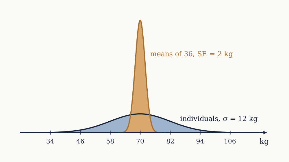
Example. Adult body mass in a population has $μ = 70$ kg and $σ = 12$ kg. A simple random sample of 36 people is taken. What is the standard error of the sample mean?

$SE = 12 / \sqrt{36} = 2$ kg. Individuals scatter by 12 kg, and means of 36 scatter by 2 kg, a sixfold reduction bought with 36 observations.

Now you. How many people are needed to bring the standard error down to 0.5 kg?

Answer

Set $12 / \sqrt{n} = 0.5$ , so $\sqrt{n} = 24$ and $n = 576$ . Four times the precision of the 36-person sample costs sixteen times the people.

The exact result for a normal population

If the population is itself normal, no approximation is needed at any $n$ . The probability course established that a sum of independent normal variables is normal, so $\overline{X}$ is exactly normal with mean $μ$ and standard deviation $σ / \sqrt{n}$ , for $n = 2$ as much as for $n = 2000$ .

That gives probabilities immediately by standardising. For the body mass example with $n = 36$ ,

P (67 \leq \overline{X} \leq 73) = P (| \frac{\overline{X} - 70}{2} | \leq 1.5) = 2 Φ (1.5) - 1 = 0.8664

so a sample of 36 lands within 3 kg of the truth about 87 times in 100. With $n = 144$ the standard error is 1, the same 3 kg becomes three standard errors, and the probability rises to 0.9973.

This is the clean case, and it is also the rare one. Body mass is roughly normal; waiting times, incomes, counts of rare events and yes-or-no answers are not. What rescues the general case is that the normality is not needed in the population at all.

The central limit theorem, put to work

The probability course proved it, and here is what it does. For independent draws from any population with finite mean $μ$ and finite variance $σ^{2}$ ,

\frac{\overline{X} - μ}{σ / \sqrt{n}} ⟶ Z

in distribution as $n$ grows, with $Z$ standard normal. The population's own shape washes out entirely, leaving a limit that depends on it only through $μ$ and $σ$ .

The practical reading is that for large enough $n$ the two exact results above can be used as approximations for any population whatsoever. That is what makes a single normal table sufficient, and it is why the normal curve appears in analyses of data that is obviously not normal, such as counts of successes or answers on a five-point scale. The claim was never that the data is normal. It is that the mean of enough of it behaves as though it were.

Two limits on the theorem are worth stating now rather than discovering later. It requires a finite variance, and distributions with infinite variance genuinely do not obey it. And it is a statement about the centre of the distribution: convergence in the far tails is much slower than convergence near the middle, so an approximation that is excellent for the middle 95 per cent can still be wrong by a factor of several in the extreme tail, which matters when the question is about rare failures.

Example. Service times at a counter are exponentially distributed with mean 4 minutes, so $σ = 4$ minutes as well. For a sample of 50 customers, estimate the probability that the mean service time exceeds 5 minutes, and compare with the exact answer.

The standard error is $4 / \sqrt{50} = 0.5657$ , so $z = (5 - 4) / 0.5657 = 1.768$ and the normal approximation gives $1 - Φ (1.768) = 0.0385$ . The sum of 50 independent exponentials has a gamma distribution, which can be computed exactly, and the true probability is 0.0460. The approximation understates the tail by about 16 per cent of its value, because the exponential is right-skewed and 50 is not many.

Now you. For 200 customers, what is the standard error, and what does the normal approximation give for the probability that the mean exceeds 4.5 minutes?

Answer

$SE = 4 / \sqrt{200} = 0.2828$ , so $z = 0.5 / 0.2828 = 1.768$ and the approximation is again 0.0385. The exact gamma answer is 0.0425, so quadrupling the sample cut the relative error of the approximation from 16 per cent to 10 per cent.

How large is large enough

The usual textbook answer is "about 30", and it is a rule of thumb that hides a wide range. The honest answer depends on how skewed the population is and on which part of the distribution matters, and it can be settled by computing exact tails for known cases.

Take an exponential population and ask how often $\overline{X}$ exceeds $μ + 1.645 σ / \sqrt{n}$ , which the normal approximation says should be 5 per cent of the time. The exact answers are 6.7 per cent at $n = 5$ , 6.4 per cent at $n = 10$ , 5.9 per cent at $n = 30$ , 5.5 per cent at $n = 100$ and 5.2 per cent at $n = 1000$ . The convergence is real and it is slow: a thousand observations from a skewed population still leaves a nominal 5 per cent tail that is actually 5.2.

Bernoulli data is worse when $p$ is extreme, because the distribution is squashed against a boundary. With $p = 0.1$ the same nominal 5 per cent upper tail is 7.3 per cent at $n = 30$ , 7.3 per cent at $n = 100$ and 5.5 per cent at $n = 300$ . The working rule from the probability course, that $n p$ and $n (1 - p)$ should both exceed about 10, is the right one, and it is a statement about $n p$ rather than about $n$ .

At the other extreme, a uniform population is symmetric and short-tailed, and the mean of just four draws is already close enough to normal for most purposes. Symmetry is what the approximation likes; skew is what it struggles with, because the leading correction term to the normal approximation is proportional to the population's skewness divided by $\sqrt{n}$ .

The standard error when the population variance is unknown

There is a circularity in everything above. The standard error $σ / \sqrt{n}$ contains $σ$ , a population parameter, and if $μ$ is unknown then $σ$ almost certainly is too. The practical move is to substitute the sample standard deviation $s$ from the second lesson, giving the estimated standard error

\hat{SE} = \frac{s}{\sqrt{n}}

This is what every piece of software reports, and it costs something. The quantity $(\overline{X} - μ) / (s / \sqrt{n})$ has a random denominator as well as a random numerator, so it is more variable than the standardised version with $σ$ in it, and its distribution has heavier tails than the normal. For large $n$ the difference is negligible because $s$ is then a precise estimate of $σ$ ; for small $n$ it is not, and the correct distribution is the $t$ , derived in the lesson on confidence intervals. Until then, the substitution is fine for $n$ in the hundreds and misleading for $n$ under about 30.

Example. A sample of 25 measurements has $\overline{x} = 12.4$ and $s = 3.0$ . Give the estimated standard error, and say what it does and does not describe.

$\hat{SE} = 3.0 / \sqrt{25} = 0.6$ . That is an estimate of how much the sample mean would move from one sample of 25 to the next. It is not an estimate of how much individual measurements vary, which is 3.0, five times as large, and it is not a bound on how wrong the mean can be if the sampling was biased.

Now you. A second sample of 100 measurements from the same population gives $s = 3.2$ . What is its estimated standard error, and how does the spread of the data compare between the two samples?

Answer

$\hat{SE} = 3.2 / \sqrt{100} = 0.32$ . The data is about as spread out in both samples, 3.0 against 3.2, as it should be since both estimate the same $σ$ . Only the standard error fell, and it fell by the factor $\sqrt{4} = 2$ that the larger sample bought.

Two distributions that must not be confused

It is worth separating the three distributions now in play, because they are routinely collapsed into one.

The population distribution is the shape of the values in the world: skewed, bimodal, discrete, whatever it happens to be. The sample distribution is the shape of the batch actually collected, which resembles the population more closely as $n$ grows and never becomes normal unless the population is. The sampling distribution of $\overline{X}$ is the shape of the estimate across hypothetical repetitions, and it becomes normal as $n$ grows regardless of the other two.

A histogram of 10,000 incomes is right-skewed and stays right-skewed no matter how much more data arrives, because it is estimating the population shape and the population is skewed. The sampling distribution of the mean of those 10,000 incomes is very nearly normal with a standard deviation 100 times smaller than the spread of the data. Both facts are true simultaneously, and a report that shows the first while quoting an interval based on the second is not contradicting itself.

With the sampling distribution in hand, the sample mean can be defended as an estimator: it is centred correctly and its spread is known. What has not been asked is whether it was the best statistic to use, or where the $n - 1$ in $s^{2}$ came from, or what to do for a parameter with no obvious sample analogue. Those are the questions of the next lesson.