Fitting a line

Comparing two groups asks whether a category changes an outcome. When the predictor is itself a number, an air temperature, a dose, a distance, grouping throws away most of the information in it. Fitting a line uses all of it, and it is the most heavily used and most heavily overinterpreted procedure in the subject.

The model, and what is random in it

Write the model as

Y_{i} = β_{0} + β_{1} x_{i} + ε_{i}

where $β_{0}$ and $β_{1}$ are unknown constants, the $x_{i}$ are treated as fixed and known, and the errors $ε_{i}$ are independent with mean zero and common variance $σ^{2}$ . The only random thing is the error, which is why $Y$ is capitalised and $x$ is not.

The assumptions packed into that line are worth naming because each can fail. The relationship is linear in the parameters. The errors have the same variance at every $x$ , called homoscedasticity. They are independent of each other. And the $x$ values are measured without error, which is often false and is the assumption people are least aware of making.

The estimates of $β_{0}$ and $β_{1}$ are written $b_{0}$ and $b_{1}$ , and they are statistics with sampling distributions like any others.

Least squares, derived

Choose the line that minimises the total squared vertical distance from the points to it:

S (b_{0}, b_{1}) = \sum_{i = 1}^{n} {(y_{i} - b_{0} - b_{1} x_{i})}^{2}

Differentiate with respect to each and set both to zero. For the intercept,

\frac{\partial S}{\partial b_{0}} = - 2 \sum_{i} (y_{i} - b_{0} - b_{1} x_{i}) = 0

which says the residuals sum to zero, so $\overline{y} = b_{0} + b_{1} \overline{x}$ : the fitted line passes through the point of means, whatever the slope is. For the slope,

\frac{\partial S}{\partial b_{1}} = - 2 \sum_{i} x_{i} (y_{i} - b_{0} - b_{1} x_{i}) = 0

Substituting $b_{0} = \overline{y} - b_{1} \overline{x}$ into that and collecting terms gives

b_{1} = \frac{\sum_{i} (x_{i} - \overline{x}) (y_{i} - \overline{y})}{\sum_{i} (x_{i} - \overline{x})^{2}} = \frac{S_{x y}}{S_{x x}}

So the slope is the sample covariance divided by the variance of $x$ . Since the correlation is $r = S_{x y} / \sqrt{S_{x x} S_{y y}}$ , an equivalent and more revealing form is

b_{1} = r \frac{s_{y}}{s_{x}}

the correlation scaled by the ratio of the two spreads. Vertical distances are minimised, not perpendicular ones, which is why regressing $y$ on $x$ and $x$ on $y$ give different lines: the second has slope $r s_{x} / s_{y}$ , and the two agree only when $| r | = 1$ .

Example. In Pearson and Lee's 1903 data on 1078 father and son pairs, fathers have mean height 67.7 inches with standard deviation 2.7, sons have mean 68.7 with the same standard deviation, and the correlation is 0.51. Find the line predicting a son's height from his father's.

The slope is $0.51 \times 2.7 / 2.7 = 0.51$ , and the intercept is $68.7 - 0.51 (67.7) = 34.17$ inches. So a father 6 inches above the mean has a son predicted only $0.51 (6) = 3.1$ inches above the mean. Francis Galton noticed exactly this in the 1880s and called it regression towards mediocrity, which is where the word "regression" comes from, and it is a consequence of $| r | < 1$ rather than a biological force.

Now you. What line predicts the father's height from the son's?

Answer

The slope is again $0.51 \times 2.7 / 2.7 = 0.51$ , with intercept $67.7 - 0.51 (68.7) = 32.66$ . The prediction runs backwards in time and still shrinks towards the mean, which shows that regression to the mean is a statement about correlation and not about inheritance or causation.

How much the line explains

Split the total variation in $y$ into what the line accounts for and what it does not. With ${\hat{y}}_{i} = b_{0} + b_{1} x_{i}$ , the identity

\sum_{i} (y_{i} - \overline{y})^{2} = \sum_{i} ({\hat{y}}_{i} - \overline{y})^{2} + \sum_{i} (y_{i} - {\hat{y}}_{i})^{2}

holds exactly, because the cross term vanishes by the two normal equations above. The three pieces are the total, regression and error sums of squares, and the ratio

r^{2} = \frac{SSR}{SST}

is the fraction of the variance of $y$ accounted for by the line. It is the square of the correlation, which is where the notation comes from.

The phrase "explained variance" is standard and misleading. A high $r^{2}$ says the points lie close to some line; it says nothing about whether the line is the right shape, whether $x$ causes $y$ , or whether the model would predict a new observation well. Anscombe's second dataset from the second lesson is an exact parabola and has $r^{2} = 0.67$ , the same as the honest linear one. A low $r^{2}$ is likewise not a failure: in a field with large individual variation, a real and important effect can account for a few per cent of the variance and still matter.

Inference on the slope

The slope is a weighted sum of the $y_{i}$ , so if the errors are independent with variance $σ^{2}$ its variance follows from adding variances:

Var (b_{1}) = \frac{σ^{2}}{S_{x x}}

Two design consequences drop out immediately. Precision improves as the $x$ values are spread further apart, since $S_{x x}$ grows, so an experiment that can choose its doses should use the extremes rather than crowding the middle. And it improves with $n$ through the same sum.

The error variance is estimated from the residuals, dividing by $n - 2$ because two parameters were estimated before the residuals were formed:

s^{2} = \frac{1}{n - 2} \sum_{i} (y_{i} - {\hat{y}}_{i})^{2}

Then $(b_{1} - β_{1}) / (s / \sqrt{S_{x x}})$ follows a $t$ distribution on $n - 2$ degrees of freedom, and intervals and tests follow exactly as before.

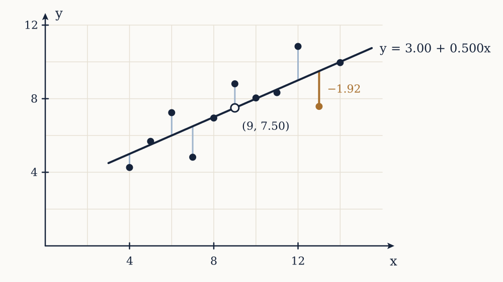
Example. Take Anscombe's first dataset, eleven points with $x$ = 10, 8, 13, 9, 11, 14, 6, 4, 12, 7, 5 and $y$ = 8.04, 6.95, 7.58, 8.81, 8.33, 9.96, 7.24, 4.26, 10.84, 4.82, 5.68. Fit the line and test whether the slope differs from zero.

Here $S_{x x} = 110$ and $S_{x y} = 55.01$ , so $b_{1} = 0.5001$ and $b_{0} = 7.5009 - 0.5001 (9) = 3.0001$ . The residual sum of squares is 13.763, so $s^{2} = 13.763 / 9 = 1.5292$ and $s = 1.237$ . Then $SE (b_{1}) = 1.237 / \sqrt{110} = 0.1179$ , giving

t = \frac{0.5001}{0.1179} = 4.24

on 9 degrees of freedom, with $p = 0.0022$ . The 95 per cent interval for the slope is $0.5001 \pm 2.262 (0.1179) = (0.233, 0.767)$ .

Now you. What is $r^{2}$ for this fit, given that the total sum of squares is 41.273?

Answer

$SSR = 41.273 - 13.763 = 27.510$ , so $r^{2} = 27.510 / 41.273 = 0.667$ , and $r = \sqrt{0.667} = 0.816$ . The line accounts for two thirds of the variation in $y$ .

Residuals are the check

Every number in the previous section is also produced, identically, by Anscombe's other three datasets, and in three of the four cases it is worthless. The check that distinguishes them is the residuals, $e_{i} = y_{i} - {\hat{y}}_{i}$ , and what to look for is specific.

Plotted against the fitted values, residuals should show no pattern. A curve means the relationship is not linear and the model is wrong in shape, which is Anscombe's second dataset. A funnel, widening as the fitted values grow, means the error variance is not constant, which often signals that the response should be modelled on a log scale. A single point far from the rest, which is Anscombe's third, means the fit is being determined by one observation.

Influence is worth separating from being an outlier. A point with an unusual $y$ but ordinary $x$ inflates the residual variance and moves the line little. A point with unusual $x$ has high leverage, because $b_{1}$ weights observations by $(x_{i} - \overline{x})$ , and if it also has an unusual $y$ it can set the slope almost by itself. That is Anscombe's fourth dataset, where ten points share one $x$ value: delete the eleventh and the slope is not merely different, it is undefined. The usual diagnostic is to refit without each point and see how much the estimates move.

Example. In the Anscombe I fit above, the residual at $x = 13$ is $- 1.92$ and the residual standard deviation is 1.237. Is this point unusual?

The standardised residual is $- 1.92 / 1.237 = - 1.55$ , well inside the range a normal error would produce in eleven observations. It is not an outlier, and with $x = 13$ against a mean of 9 it has moderate leverage, so it is worth noting rather than acting on.

Now you. The fitted value at $x = 10$ is 8.00 and the observed $y$ is 8.04. What is the standardised residual?

Answer

$0.04 / 1.237 = 0.03$ , essentially on the line.

Prediction, and the edge of the data

A fitted line supports two different intervals at a new $x$ , and confusing them is common. The interval for the mean response at $x_{0}$ has width driven by the uncertainty in $b_{0}$ and $b_{1}$ alone. The interval for a single new observation at $x_{0}$ must additionally include the error term $ε$ , so its variance is larger by $σ^{2}$ and it is much wider. A regression with $r^{2} = 0.99$ can still predict an individual case poorly.

Both intervals widen as $x_{0}$ moves away from $\overline{x}$ , because a small error in the slope is amplified by the lever arm. Beyond the range of the data, the widening is the least of the problems: there the model itself is an untested guess, and no interval accounts for the possibility that the relationship bends.

Edwin Hubble's 1929 paper fitted a line to the velocities and distances of 24 galaxies and obtained a slope of about 500 kilometres per second per megaparsec. The modern value is near 70. The regression arithmetic was not wrong: the distances fed into it were wrong, by a factor of about seven, because the calibration of the distance indicators was. This is the assumption that $x$ is measured without error, failing in the most consequential way, and it is not visible anywhere in the residual plots.

What a slope is not

A fitted slope says that, in this sample, $y$ is on average higher by $b_{1}$ for each unit of $x$ . It does not say that changing $x$ would change $y$ , and the gap between those two sentences is where most misuse of regression happens.

Three things can produce a slope with no causal content. The relationship may run the other way, since least squares is symmetric about which variable is called the response. A third variable may drive both, which the fitted line has no way to detect. Or the sample may have been assembled so as to create the association, as when only cases meeting some combined criterion are recorded.

Nothing in this lesson distinguishes those from a genuine causal effect, because nothing in the data can. What does distinguish them is how the data was produced, which is the next lesson.