Describing a batch of numbers

A sample of a thousand measurements cannot be thought about all at once, so the first act of any analysis is to replace it with a few numbers. The previous lesson called those numbers statistics and said they were random; this one asks which ones to compute, and shows that the choice is a substantive decision rather than a formality.

What a summary is for

There are two different jobs on offer. One is description: saying compactly what this batch looks like, with no claim about anything beyond it. The other is estimation: using the batch to guess a property of the population it came from. The same arithmetic serves both, which is why they get muddled, but the standards differ. A description is right or wrong about the data in front of it, while an estimate can be an accurate description and still a bad guess.

The running example is real and small enough to check by hand. In 1798 Henry Cavendish published 29 determinations of the mean density of the Earth, relative to water, from the tiny attraction between lead spheres on a torsion balance. Sorted, they are

4.88, 5.07, 5.10, 5.26, 5.27, 5.29, 5.29, 5.30, 5.34, 5.34, 5.36, 5.39, 5.42, 5.44, 5.46, 5.47, 5.50, 5.53, 5.55, 5.57, 5.58, 5.61, 5.62, 5.63, 5.65, 5.68, 5.75, 5.79, 5.85

The modern value is 5.514, so this batch is a rare case where the truth is known and the quality of each summary can be judged against it.

Where the middle is

The sample mean is the total shared out equally,

\overline{x} = \frac{1}{n} \sum_{i = 1}^{n} x_{i}

which for Cavendish's 29 values is 5.448. The median is the middle value once sorted, the fifteenth here, which is 5.46. They differ by 0.012, and the reason is the first value in the list.

Each of the two is the answer to a precise optimisation, which is the honest way to see what distinguishes them. Ask which single number $c$ makes the total squared error $\sum (x_{i} - c)^{2}$ as small as possible. Differentiate: $\frac{d}{d c} \sum (x_{i} - c)^{2} = - 2 \sum (x_{i} - c)$ , which vanishes when $\sum x_{i} = n c$ , so $c = \overline{x}$ , and the second derivative $2 n$ is positive so it is a minimum. The mean is the least-squares centre.

Now ask which $c$ minimises the total absolute error $\sum | x_{i} - c |$ . Each term contributes a slope of $- 1$ while $c$ is below $x_{i}$ and $+ 1$ while it is above, so the total slope is (number of points below $c$ ) minus (number above). That is zero exactly when the two counts balance, which is the definition of the median. The median is the least-absolute-error centre.

The difference between squaring an error and not squaring it is the whole story. Squaring makes a point ten times as far away count a hundred times as much, so the mean is dragged towards any distant value, while the median counts only which side each point falls on and so ignores how far out it is.

Example. Seven employees earn 21, 23, 24, 26, 28, 30 and 210 thousand pounds. Find the mean and the median, and say which better describes what a typical employee earns.

The total is 362, so $\overline{x} = 362 / 7 = 51.7$ thousand. The median is the fourth of the seven sorted values, 26 thousand. Six of the seven employees earn less than the mean, so as a description of a typical wage the mean is useless here and the median is exact. As a description of the payroll the mean is the right one: it is the total divided by the headcount, and the total is what the employer pays.

Now you. The employee on 210 leaves and is not replaced. Find the new mean and median.

Answer

The remaining six total 152, so the mean is $152 / 6 = 25.3$ thousand, a fall of 26.4. The median becomes the average of the third and fourth values, $(24 + 26) / 2 = 25$ , a fall of 1. One departure moved the mean by more than a quarter of its value and the median by four per cent.

Quantiles and the five-number summary

The median generalises. The quantile at level $q$ is a value with a fraction $q$ of the data at or below it, so the median is the quantile at 0.5, the quartiles are at 0.25 and 0.75, and percentiles are quantiles expressed in hundredths. For a finite batch the definition needs a tie-breaking convention when $q n$ is not a whole number, and software packages use at least nine different ones, so quartiles quoted to three decimals from different tools will not always agree. The convention used here is the simplest: the median of the values below the median, and the median of the values above it.

For Cavendish that gives $Q_{1} = 5.295$ and $Q_{3} = 5.615$ , so the middle half of his measurements spans 0.32. Together with the smallest value 4.88, the median 5.46 and the largest 5.85, those five numbers are the five-number summary, and they are what a boxplot draws.

The distance $Q_{3} - Q_{1}$ is the interquartile range, and it is the natural partner of the median: both depend only on the ordering of the data, and neither notices how extreme an extreme value is. A common convention flags as outliers any point more than $1.5 \times IQR$ beyond a quartile. Here that means below $5.295 - 0.48 = 4.815$ or above $5.615 + 0.48 = 6.095$ , and Cavendish's suspicious 4.88 falls inside the lower fence and is not flagged. The rule is a convention, chosen because it flags about 0.7 per cent of a normal sample, and it has no authority to declare a measurement wrong.

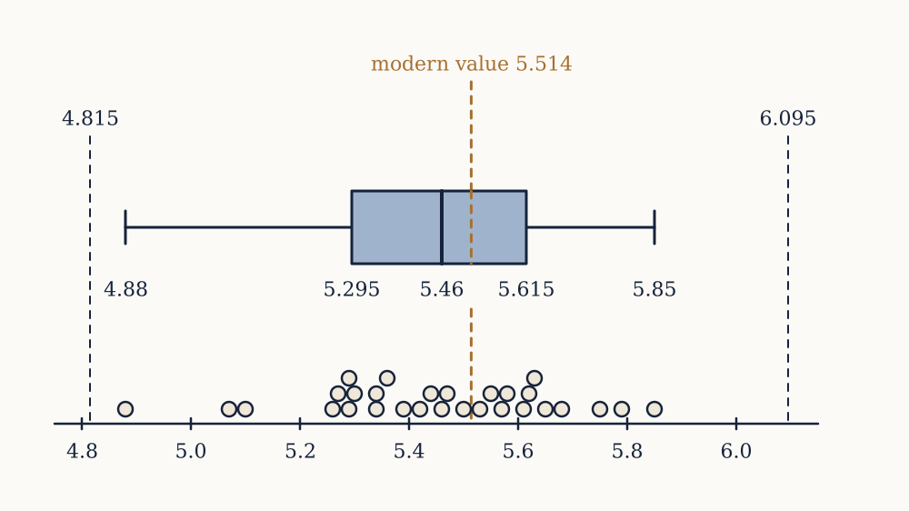
Example. For the Cavendish batch, what fraction of the values lie within the interquartile range, and what does that say about the shape?

By construction about half do, which is what makes the IQR comparable across batches. What is informative is the position of the median inside it: $5.46 - 5.295 = 0.165$ below and $5.615 - 5.46 = 0.155$ above, almost symmetric, so the middle of this batch is not skewed even though the lowest value sits well out.

Now you. Using the same $1.5 \times IQR$ convention, how far below $Q_{1}$ would a measurement have to fall to be flagged?

Answer

Below $5.295 - 1.5 (0.32) = 4.815$ . Cavendish's 4.88 misses the fence by 0.065, which is why a summary should never be the only thing looked at.

Measuring spread

Location without spread is nearly useless: two batches with the same centre can be entirely different. The natural measure of spread starts from the deviations $x_{i} - \overline{x}$ , whose sum is always exactly zero by the least-squares property above, so they must be squared before adding. The sample variance is

s^{2} = \frac{1}{n - 1} \sum_{i = 1}^{n} (x_{i} - \overline{x})^{2}

and the sample standard deviation $s$ is its square root, which restores the original units. For Cavendish, $s = 0.221$ .

The divisor is $n - 1$ rather than $n$ , and the reason is genuinely not obvious. The short version is that the deviations are taken from $\overline{x}$ rather than from the true mean, and $\overline{x}$ sits by construction in the middle of this particular sample, so the squared deviations come out systematically too small. Dividing by $n - 1$ corrects that exactly. The lesson on estimators proves it; for now, treat $n - 1$ as the version to use whenever the batch is a sample from something larger, which is essentially always.

The standard deviation has the same units as the data and scales the same way. Adding a constant to every value shifts the mean by that constant and leaves $s$ untouched, since it shifts every deviation equally by zero. Multiplying every value by $a$ multiplies the mean by $a$ and the standard deviation by $| a |$ , so converting a batch of prices from pounds to pence multiplies both by 100. That is why a standard deviation is meaningless without its units, and why the dimensionless ratio $s / \overline{x}$ , the coefficient of variation, is the right thing to quote when comparing spreads across quantities of different sizes.

Example. Find the mean, variance and standard deviation of 2, 4, 4, 4, 5, 5, 7, 9.

The total is 40 and $n = 8$ , so $\overline{x} = 5$ . The deviations are $- 3, - 1, - 1, - 1, 0, 0, 2, 4$ , whose squares total $9 + 1 + 1 + 1 + 0 + 0 + 4 + 16 = 32$ . So $s^{2} = 32 / 7 = 4.571$ and $s = 2.138$ . Dividing by 8 instead would give exactly 4 and 2, which is why this batch appears in textbooks, and why it quietly teaches the wrong divisor.

Now you. Every value is doubled, giving 4, 8, 8, 8, 10, 10, 14, 18. What are the new variance and standard deviation?

Answer

Doubling multiplies the standard deviation by 2 and the variance by 4, so $s^{2} = 18.29$ and $s = 4.276$ . No fresh arithmetic is needed.

Resistance against efficiency

There is now a mean and a median, a standard deviation and an interquartile range, and a standing question of which to use. The trade is between resistance and efficiency, and it is real in both directions.

An estimator is resistant if a small number of arbitrarily bad values cannot move it far. The median's breakdown point is 50 per cent: half the data can be replaced by nonsense before the median leaves the range of the good half. The mean's breakdown point is $1 / n$ , since one value taken to infinity takes the mean with it. The employee example showed a breakdown point of one seventh in action. Removing Cavendish's 4.88 moves the mean from 5.448 to 5.468 and the median from 5.46 to 5.465, a factor of four difference in sensitivity from a single point out of 29.

Resistance is not free. If the data really is a clean sample from a normal population, the median throws away information: its sampling variance is $π / 2 \approx 1.57$ times that of the mean for large $n$ , so using the median costs about 36 per cent of the sample. A study of 1000 people analysed by medians has the precision of one of 640 analysed by means, which is an expensive kind of caution.

The working rule that follows is not a formula but a habit. Use the mean and standard deviation when the batch is roughly symmetric and free of stragglers, since they are more precise and everything downstream in this course is built on them. Use the median and interquartile range when the batch is skewed or contaminated, and say which was used. Quoting both, and noting when they disagree, tells the reader more than either alone: the gap between them is itself a measurement of skew.

Shape, and why the mean and median part company

When the mean sits well above the median, a long right tail is pulling it. United States household income in 2022 had a median of 74,580 dollars and a mean of 105,555 dollars, a ratio of 1.42, and the mechanism is the same as in the payroll example on a national scale. Reporting the mean is not wrong, but it answers "how much income is there per household", not "what does a household in the middle have", and the two questions have politically different answers.

Skew is measured formally by the third standardised moment, $\frac{1}{n} \sum (x_{i} - \overline{x})^{3} / s^{3}$ , zero for a symmetric batch, positive for a right tail and negative for a left one. Cubing makes it even more sensitive to single extreme points than the variance is, so it is worth knowing and worth distrusting.

The more useful move with strongly right-skewed data is to take logarithms first. If the values are generated multiplicatively, incomes, city populations, particle sizes, then their logarithms are roughly symmetric and everything in this course applies to those instead. The mean of the logarithms exponentiates back to the geometric mean, the correct centre for quantities that compound.

What summaries cannot see

In 1973 Francis Anscombe published four datasets of eleven points each, constructed so that a great deal of standard arithmetic cannot tell them apart. All four have $\overline{x} = 9.00$ , $\overline{y} = 7.50$ , sample variance of $x$ equal to 11.00, sample variance of $y$ equal to 4.13, correlation 0.816, and least squares line $y = 3.00 + 0.500 x$ , all agreeing to the printed precision.

The first is a genuine noisy linear relationship, which is what everyone pictures. The second is a perfect parabola, with no straight-line relationship at all, that the fitted line describes catastrophically. The third is eleven points in an exact straight line of different slope plus a single far-off point that drags the fit to match the first two. The fourth has ten points sharing one $x$ value and a single point elsewhere, so the entire slope is determined by one observation, and deleting it leaves the slope undefined.

The lesson usually drawn is "plot the data", which is correct and slightly too comfortable. The sharper version is that these summaries are answers to specific questions, and a batch is not obliged to be the kind of thing those questions are about. The mean of a bimodal batch describes a value that may occur in neither mode. A correlation summarises linear association and returns something meaningless when the relationship is not linear. The failure is not in the arithmetic, which is exact, but in the assumption that the arithmetic was worth doing.

Every number so far has described the batch in hand. Whether any of them says anything about the world depends entirely on how the batch was collected, which is the next lesson, and no amount of care with quartiles repairs a sample chosen badly.