The normal curve

Four distributions in this course came from four different mechanisms and have four different shapes. A fifth shape appears in measurement after measurement without any obvious mechanism behind it at all, and this lesson takes it as given, learns to compute with it, and is honest about where it does not belong. Why it is unavoidable is the next lesson.

The curve and its two parameters

The normal or Gaussian density is

f (x) = \frac{1}{σ \sqrt{2 π}} e^{- (x - μ)^{2} / (2 σ^{2})}

and although it looks arbitrary, each piece has a job. The exponent is a negative multiple of the squared distance from $μ$ , so the curve is symmetric about $μ$ and falls away in both directions. It falls extremely fast, because the exponent grows with the square of the distance, and this is what makes the tails so thin. The $σ^{2}$ in the denominator of the exponent sets the horizontal scale, so the curve is wide when $σ$ is large. The factor in front is fixed by the requirement that the total area equal $1$ , and the $\sqrt{2 π}$ is the constant that makes it so, a result from calculus that this course takes on trust.

The parameters are exactly the mean and the standard deviation, both of which follow from the symmetry and from an integral. So a normal distribution is completely determined by its first two moments, which is a strong and unusual property: for a binomial you also need $n$ and $p$ separately, and for most families two numbers do not fix the shape.

Abraham de Moivre found the curve in 1733 as an approximation to the binomial for large $n$ , in a private pamphlet, and it lay unused. Carl Friedrich Gauss arrived at it again in 1809 from a completely different direction, asking what error distribution would make the arithmetic mean the best estimate of a measured quantity, and found this one. Two unrelated routes to the same curve was the first hint that something general was going on.

One curve, one table

The density has no elementary antiderivative, so areas under it cannot be written in closed form and must be looked up or computed numerically. Doing that separately for every $μ$ and $σ$ would be hopeless, and the scaling rule from the variance lesson removes the need. Standardise:

Z = \frac{X - μ}{σ}

which has mean $0$ and variance $1$ , and which is still normal, because subtracting and dividing by constants only shifts and stretches the curve. So every normal question reduces to a question about the standard normal, whose cumulative function is written $Φ (z)$ . One table, or one library function, serves every case.

The recipe is mechanical. To find $P (X \leq x)$ , compute $z = (x - μ) / σ$ and read $Φ (z)$ . To find a probability between two values, subtract. For the upper tail use $1 - Φ (z)$ , and use the symmetry $Φ (- z) = 1 - Φ (z)$ to avoid needing negative arguments at all.

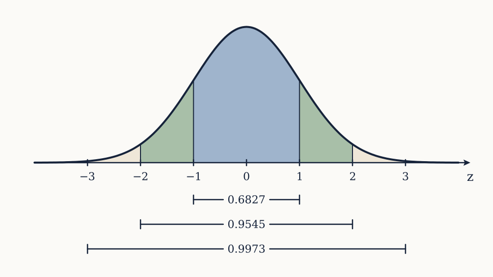
The figures everyone quotes come straight out of this. The area within one standard deviation of the mean is $Φ (1) - Φ (- 1) = 2 Φ (1) - 1 = 0.682689$ . Within two it is $0.954500$ , within three $0.997300$ , and within four $0.999937$ . Rounded, that is the $68$ , $95$ , $99.7$ rule, and it is worth noticing how brutal the decay is: the chance of landing beyond four standard deviations is about $1$ in $15800$ , and beyond five about $1$ in $1.7$ million. Compare Chebyshev's guarantee from the earlier lesson, which allowed up to $1 / 9$ beyond three standard deviations for an arbitrary distribution against the normal's $0.0027$ . Assuming normality buys enormous precision in the tails, and losing that assumption is expensive in exactly the same place.

Example. A population of adult men has mean height $175$ cm with standard deviation $7$ cm, close to the figures reported for England. What proportion are taller than $190$ cm?

Standardise: $z = (190 - 175) / 7 = 2.1429$ . Then $Φ (2.1429) = 0.98394$ , so the upper tail is $1 - 0.98394 = 0.01606$ , about $1.6$ percent, or one man in $62$ .

Now you. For the same population, what proportion are between $168$ and $182$ cm tall?

Answer

Those bounds are exactly one standard deviation either side of the mean, so the answer is $2 Φ (1) - 1 = 0.6827$ , about $68$ percent.

Reading the table backwards

The recipe above answers "what fraction lies beyond this value". The reverse question, "what value has this fraction beyond it", is answered by running $Φ$ backwards, and it is the form most decisions take.

Two values are worth memorising because they appear everywhere. $Φ (1.645) = 0.95$ , so five percent of a normal distribution lies above $1.645$ standard deviations from the mean. And $Φ (1.96) = 0.975$ , so two and a half percent lies above $1.96$ standard deviations and, by symmetry, ninety-five percent lies within $\pm 1.96$ . That second figure is where the ubiquitous " $1.96$ " in confidence intervals and polling margins comes from, and the next lesson derives that use of it in full.

Converting back to the original units is the scaling rule in reverse: the value with fraction $q$ below it is $x_{q} = μ + z_{q} σ$ . For the height population above, the ninety-fifth percentile is $175 + 1.645 (7) = 186.5$ cm, and the fifth percentile is $175 - 1.645 (7) = 163.5$ cm. A design that must fit ninety-five percent of the population is sized to the first of those, and the five percent it excludes are the price of the choice, stated rather than hidden.

Percentile talk is normal-curve talk in disguise wherever it is used on test scores, growth charts and reference ranges. The clinical convention of flagging results outside the central ninety-five percent of a reference population is exactly the $\pm 1.96$ rule, and it guarantees that one healthy person in twenty is flagged, which is the multiple comparisons problem of the last lesson waiting to happen.

Normal plus normal is normal

One property makes the normal indispensable in practice: independent normal variables add to a normal variable. If $X$ is normal with mean $μ_{1}$ and variance $σ_{1}^{2}$ , and $Y$ is independent normal with $μ_{2}$ and $σ_{2}^{2}$ , then $X + Y$ is normal with mean $μ_{1} + μ_{2}$ and variance $σ_{1}^{2} + σ_{2}^{2}$ .

The means and variances combining that way is nothing new, since linearity and independent additivity were proved for all variables. What is new is that the shape is preserved. Add two uniforms and you get a triangle, not a uniform. Add two exponentials and you get something with a peak away from zero. The normal is a fixed point of addition, and combined with the fact that it approximates so much else, that is why it propagates through any calculation that adds things up.

Example. A component's length is normal with mean $50.0$ mm and standard deviation $0.3$ mm. Four are stacked end to end, independently. What is the distribution of the total length, and what fraction of stacks exceed $201$ mm?

The total is normal with mean $200.0$ mm and variance $4 (0.09) = 0.36$ , so its standard deviation is $0.6$ mm, not $1.2$ mm. Then $z = (201 - 200) / 0.6 = 1.6667$ , so the fraction above is $1 - Φ (1.6667) = 0.0478$ , about $4.8$ percent.

Now you. Nine such components are stacked. What are the mean and standard deviation of the total length?

Answer

Mean $450.0$ mm. Variance $9 (0.09) = 0.81$ , so the standard deviation is $0.9$ mm. Nine times the components, three times the spread.

Approximating the binomial

De Moivre's original purpose still works, and it is the practical way to handle a binomial with large $n$ . A $Bin (n, p)$ variable has mean $n p$ and variance $n p (1 - p)$ , and for large $n$ its mass function is closely matched by the normal curve with those parameters.

One adjustment is needed. The binomial is discrete and the normal is continuous, so a bar of the mass function at $k$ is represented by the strip of normal area from $k - 0.5$ to $k + 0.5$ . Using those half-unit boundaries is the continuity correction, and skipping it is the usual source of a poor approximation.

Take $100$ fair coin tosses and ask for $P (X \geq 60)$ . The mean is $50$ and the standard deviation is $\sqrt{100 \times 0.25} = 5$ . With the correction, the boundary is $59.5$ , so $z = (59.5 - 50) / 5 = 1.9$ and the tail is $1 - Φ (1.9) = 0.028717$ . The exact binomial answer is $0.028444$ , so the error is under one percent of the value. Without the correction the boundary would be $60$ , giving $z = 2$ and $0.02275$ , which is wrong by twenty percent. The correction is not a refinement, it is the difference between a usable answer and a bad one.

The approximation is good when $n p$ and $n (1 - p)$ both comfortably exceed about $10$ , which keeps the binomial from being squashed against either boundary. When $p$ is tiny and $n p$ is small, the right approximation is the Poisson of the earlier lesson instead.

Example. A fair coin is tossed $100$ times. Estimate the probability that the number of heads differs from $50$ by at least $15$ , and compare with the exact value.

The boundaries with continuity correction are $50 \pm 14.5$ , so $z = 14.5 / 5 = 2.9$ and the two-sided tail is $2 (1 - Φ (2.9)) = 0.003732$ . The exact binomial value is $0.003518$ . Chebyshev, for the same question, allowed anything up to $0.1111$ .

Now you. For the same $100$ tosses, estimate $P (X \geq 55)$ using the normal approximation with continuity correction.

Answer

The boundary is $54.5$ , so $z = 4.5 / 5 = 0.9$ and the answer is $1 - Φ (0.9) \approx 0.1841$ . The exact binomial value is $0.1841$ as well, to four places.

Where the curve does not belong

The normal is a model, and it is applied far outside the range where it is warranted. Three failures are worth being able to spot.

The curve extends to infinity in both directions, so a normal model always assigns positive probability to negative values. For heights with mean $175$ cm and standard deviation $7$ cm, negative height is twenty-five standard deviations out and the probability is unimaginably small, so the defect is harmless. For a quantity whose mean is close to zero relative to its spread, such as a rainfall total or a waiting time, the defect is fatal, and the model will predict impossible outcomes at a noticeable rate.

Second, the tails are extraordinarily thin, and many real quantities have tails that are not. Daily returns on financial assets are the standard example: moves of more than five standard deviations should occur roughly once in $7000$ years of trading days under a normal model, and they occur every few years. Insurance losses, city sizes, file sizes and word frequencies behave similarly. Fitting a normal to such data produces a model that is comfortable, tractable and wrong precisely about the events that matter, which is worse than having no model.

Third, quantities generated by multiplication rather than addition are not normal but log-normal: their logarithm is normal, and their own distribution is skewed right with a long tail. Incomes, particle sizes and biological growth often behave this way, since the next value is the previous one times a random factor. The tell is a distribution whose mean noticeably exceeds its median.

A good habit is to ask why the quantity should be normal before assuming it is. The honest answer is usually that it is a sum of many small independent contributions, and that answer is a theorem rather than a hope. Stating that theorem, and the companion result about why averages settle down at all, is the next lesson.