Bayes' theorem

The conditional probabilities that are easy to state run from cause to observation, and the ones people actually want run the other way. This lesson derives the formula that turns one into the other, applies it to a real screening test where the honest answer is startling, and shows why the result is so consistently misjudged, including by the professionals who depend on it.

Turning the conditional around

The previous lesson defined $P (A | B) = P (A \cap B) / P (B)$ , and the intersection can be expanded in either order:

P (A \cap B) = P (B) P (A | B) = P (A) P (B | A)

Set the two right-hand sides equal and divide by $P (B)$ , which is legitimate whenever $P (B) > 0$ :

P (A | B) = \frac{P (A) P (B | A)}{P (B)}

That is Bayes' theorem, published posthumously in 1763 from an essay by Thomas Bayes and given its general form by Laplace in 1774. The derivation is two lines of algebra with no new assumption, which is worth stressing: nothing about the theorem is contentious. What is contentious is what people are willing to put into it.

The names for the pieces carry the meaning. Write $H$ for a hypothesis and $E$ for the evidence. Then $P (H)$ is the prior, what the hypothesis was worth before the evidence; $P (E | H)$ is the likelihood, how well the hypothesis predicts the evidence; $P (E)$ is the probability of the evidence under all hypotheses together; and $P (H | E)$ is the posterior, what the hypothesis is worth after. The denominator is almost never given directly and is nearly always computed by the law of total probability. With two hypotheses, $H$ and its negation,

P (H | E) = \frac{P (H) P (E | H)}{P (H) P (E | H) + P (H^{c}) P (E | H^{c})}

Every term on the right has an operational meaning, and the third one, $P (E | H^{c})$ , the chance of the same evidence when the hypothesis is false, is the term that gets left out when people reason informally. Evidence that fits your hypothesis is worthless unless it fits the alternatives worse.

A test that is right nine times in ten

David Eddy put the following to a group of physicians in 1978. Among women aged forty with no symptoms, about $1$ percent have breast cancer. Mammography detects it in $79.2$ percent of the women who have it, and returns a positive result for $9.6$ percent of the women who do not. A woman in this group has a positive mammogram. What is the probability that she has cancer?

Ninety-five of the hundred physicians answered around $75$ percent. The correct answer is

P (C | +) = \frac{0.01 \times 0.792}{0.01 \times 0.792 + 0.99 \times 0.096} = \frac{0.00792}{0.00792 + 0.09504} = \frac{0.00792}{0.10296} \approx 0.0769

about $7.7$ percent, off by a factor of ten. The test is not bad; the base rate is doing the damage. Only one woman in a hundred has the disease, so the $9.6$ percent false positive rate is applied to ninety-nine times as many women as the $79.2$ percent detection rate, and it wins on volume.

Nothing about this depends on medicine. Any test for a rare condition behaves this way, and the rarer the condition the worse it gets. Screen for something present in one person in ten thousand with a test that is $99$ percent sensitive and gives $1$ percent false positives, and a positive result leaves the probability at $0.0098$ , still under one percent. This is why mass screening for rare conditions is a hard policy problem rather than an obvious good, and why confirmatory tests exist.

Example. A drug test detects doping in $99$ percent of dopers and returns a positive for $2$ percent of clean athletes. Five percent of athletes in a sport dope. An athlete tests positive. What is the probability that they doped?

P (D | +) = \frac{0.05 \times 0.99}{0.05 \times 0.99 + 0.95 \times 0.02} = \frac{0.0495}{0.0495 + 0.019} = \frac{0.0495}{0.0685} \approx 0.7226

About $72$ percent, high enough to investigate and nowhere near high enough to convict on its own.

Now you. In a different sport only $1$ percent of athletes dope, with the same test. What is the probability that a positive athlete doped?

Answer

\frac{0.01 \times 0.99}{0.01 \times 0.99 + 0.99 \times 0.02} = \frac{0.0099}{0.0099 + 0.0198} = \frac{0.0099}{0.0297} \approx 0.3333

One third. The same test, the same accuracy, a base rate five times lower, and the conclusion flips from probable to unlikely.

Counting people instead of multiplying fractions

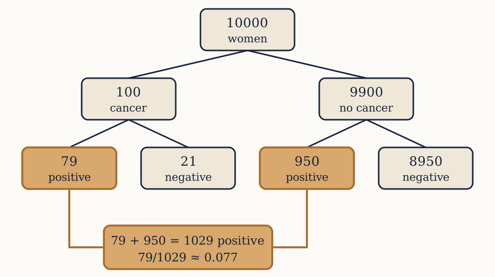
Gerd Gigerenzer showed in the 1990s that the same physicians who fail with percentages mostly succeed when the identical problem is posed in counts, and the reformulation is worth adopting permanently because it makes the answer visible without any formula.

Take $10000$ women. About $100$ of them have cancer, and of those, $79$ test positive. The other $9900$ do not have cancer, and $950$ of them test positive anyway. So $79 + 950 = 1029$ women test positive in total, of whom $79$ have cancer:

\frac{79}{1029} \approx 0.077

the same answer, reached by dividing one count by another. The version with percentages hides the fact that the two groups being compared are of wildly different sizes; the version with counts puts the $9900$ on the page where it cannot be forgotten. When you want to sanity-check any Bayes calculation, do it this way, with a round population and whole people.

Odds and the weight of evidence

There is a form of the theorem in which the awkward denominator disappears. Write Bayes for $H$ and for $H^{c}$ with the same evidence and divide one by the other. The $P (E)$ cancels, leaving

\frac{P (H | E)}{P (H^{c} | E)} = \frac{P (H)}{P (H^{c})} \times \frac{P (E | H)}{P (E | H^{c})}

In words: posterior odds equal prior odds times the likelihood ratio. Odds of $p$ against $1 - p$ convert back to a probability by $p = odds / (1 + odds)$ .

The likelihood ratio is the entire contribution of the evidence, and it is a property of the test alone, free of the base rate. For the mammogram it is $0.792 / 0.096 = 8.25$ : a positive result multiplies the odds by $8.25$ , whoever is tested and whatever they believed beforehand. That is the honest summary of what a test is worth, and it explains the earlier result at once. Prior odds of cancer are $1$ to $99$ , or $0.0101$ . Multiply by $8.25$ to get posterior odds of $0.0833$ , and convert: $0.0833 / 1.0833 \approx 0.0769$ . Multiplying odds by $8.25$ sounds impressive and moves a probability of $0.01$ only to $0.077$ , because odds far from one are hard to shift.

Repeated independent tests multiply their likelihood ratios, which makes sequential updating trivial. Two independent positive mammograms give odds $0.0101 \times {8.25}^{2} = 0.6875$ , a probability of $0.4074$ . Three give odds $5.672$ and a probability of $0.8501$ . Note also that the order of the evidence never appears in the product, so updating on $E_{1}$ then $E_{2}$ gives exactly what updating on $E_{2}$ then $E_{1}$ gives, and both equal updating on both at once. A Bayesian cannot be led anywhere by the sequencing of the evidence, only by its content.

Example. A blood test has likelihood ratio $12$ for a positive result. A patient's prior probability of the condition is $0.05$ . What is the posterior probability after one positive?

Prior odds are $0.05 / 0.95 = 0.05263$ . Multiply by $12$ to get $0.6316$ . Convert back: $0.6316 / 1.6316 \approx 0.3871$ , so about $39$ percent.

Now you. The same patient tests positive a second time, independently. What is the probability now?

Answer

Multiply the odds by $12$ again: $0.6316 \times 12 = 7.579$ , giving $7.579 / 8.579 \approx 0.8834$ , about $88$ percent.

Negative results and the other error

A test has two ways of being wrong, and the odds form handles the second as easily as the first. The likelihood ratio for a negative result is $P (- | H) / P (- | H^{c})$ , which for the mammogram is $(1 - 0.792) / (1 - 0.096) = 0.208 / 0.904 = 0.2301$ . A negative multiplies the odds by $0.23$ , cutting them by more than a factor of four.

Starting from prior odds of $1$ to $99$ , a negative mammogram gives odds $0.0101 \times 0.2301 = 0.002324$ , a probability of $0.002319$ , down from $0.01$ . So the test does useful work in both directions: it takes a one-in-a-hundred risk down to about one in four hundred and thirty. A likelihood ratio near $1$ , in either direction, is the signature of a test not worth doing, since it leaves the odds where it found them.

Example. For the drug test above, what is the likelihood ratio of a negative result, and what does a negative do to an athlete whose prior probability of doping was $0.05$ ?

The ratio is $(1 - 0.99) / (1 - 0.02) = 0.01 / 0.98 = 0.010204$ . Prior odds $0.05 / 0.95 = 0.05263$ , so posterior odds are $0.000537$ and the probability is $0.000537$ , roughly one in $1863$ .

Now you. A test has sensitivity $0.95$ and false positive rate $0.10$ . What are its likelihood ratios for a positive and for a negative result?

Answer

Positive: $0.95 / 0.10 = 9.5$ . Negative: $(1 - 0.95) / (1 - 0.10) = 0.05 / 0.90 \approx 0.0556$ , which is a division of the odds by about $18$ .

What the theorem cannot give you

Bayes' theorem is a rule for revising a probability. It is not a rule for having one in the first place, and the prior has to come from somewhere outside it. In the mammography problem the prior was a measured population rate, which is uncontroversial. In a courtroom, or in assessing a scientific hypothesis, there is no population to count, and the prior is a judgement. Two honest people with different priors will reach different posteriors from the same evidence, and the theorem cannot arbitrate between them.

What it does guarantee is that they converge under enough evidence. Each new independent observation multiplies both people's odds by the same likelihood ratio, so a disagreement of a factor of a hundred in the prior is erased by evidence worth a factor of a hundred, and strong evidence swamps any prior that was not dogmatic. The exception is a prior of exactly $0$ or $1$ , which multiplication can never move: certainty is not a strong opinion but an unreachable one, and this is the mathematical content of the advice to never be completely sure.

The theorem also silently assumes that the hypotheses listed are exhaustive. The denominator sums over the alternatives you thought of, so if the true explanation is not in the list, the posterior is confidently wrong. A high posterior means "best of what was considered", not "true".

So far every hypothesis and every event has been a yes-or-no affair. Most quantities of interest are not: how many defective items in a batch, how long until a component fails, how far a measurement is from its target. Attaching a number to each outcome, and asking what that number does on average, is the next step.