Costs

The previous lesson found the cheapest way to make any given output, and doing that at every output level is what a cost function is.

Cost is where the physical description of a firm meets the decision it actually has to take, and getting the accounting right matters more here than anywhere else in the course. A firm that measures its costs the way its accountant does will systematically reach the wrong answer about whether to stay open, and the reason goes back to the first lesson.

Economic cost is opportunity cost

The cost of a decision is what is given up because of it, which means every resource the firm uses is charged at what it could have earned elsewhere, whether or not a cheque changes hands. Accounting cost records payments. Economic cost records sacrifices, and the two differ by the implicit costs: the resources the firm owns.

Take a shop with revenue of £180,000. It pays £90,000 for stock and £30,000 for staff, so its accounting profit is £60,000. But the owner works there full time and could earn £45,000 elsewhere, and the premises are owned outright though they would rent for £20,000. Economic cost is therefore £185,000 and the economic profit is minus £5,000. The business makes an accounting profit and destroys value, and only the second number answers the question of whether to continue.

The convention that comes with this is worth knowing because it sounds strange at first. The return an owner needs to keep resources in the business is counted as a cost, so zero economic profit is a perfectly satisfactory outcome, sometimes called normal profit. When the competition lessons conclude that free entry drives profit to zero, they are not predicting that everyone goes broke; they are predicting that the owners earn exactly what their capital and effort would earn elsewhere, and no more.

Fixed, variable and sunk

In the short run some inputs cannot be varied, so total cost splits: $C (q) = F + V (q)$ , with fixed cost $F$ independent of output and variable cost $V (q)$ rising with it. Fixed cost is paid even at zero output, which is why a factory idle for a month still has a rent bill.

Sunk is a different distinction and gets confused with fixed constantly. A fixed cost is unavoidable in the short run given that the firm operates; a sunk cost is unrecoverable whatever the firm does. A year's rent on a lease that can be sublet is fixed but not sunk. Money spent on a bespoke machine with no resale value is sunk. The distinction decides which costs enter a decision at all: sunk costs enter none of them, as the first lesson argued, while fixed costs do enter the decision to shut down.

Four averages follow, and their notation is standard: average fixed cost $AFC = F / q$ , average variable cost $AVC = V (q) / q$ , average total cost $ATC = C (q) / q$ , and marginal cost $MC = d C / d q$ . Note that marginal cost contains no fixed component at all, since $F$ differentiates to zero. Marginal cost is a property of the variable input alone.

Marginal cost comes from marginal product

Cost curves are not free-standing; they are the production function seen through input prices. Suppose labour is the only variable input at wage $w$ . Producing one more unit of output requires $1 / {MP}_{L}$ extra workers, each costing $w$ , so

MC = \frac{w}{{MP}_{L}}

Marginal cost is the wage divided by the marginal product. That single equation explains the shape of every short-run cost curve in the subject: where marginal product rises, marginal cost falls, and where diminishing marginal returns set in, marginal cost turns upward. The U-shape of the cost curves is the inverted image of the hump in the product curves, not an independent assumption. By the same argument $AVC = w / {AP}_{L}$ .

Example. The workshop from the previous lesson has $q = 30 L^{2} - L^{3}$ and pays £600 a week per worker. Find marginal cost at $L = 10$ and at $L = 18$ .

The marginal product is $60 L - 3 L^{2}$ , which is 300 at $L = 10$ and 108 at $L = 18$ . So marginal cost is $600 / 300 = £ 2$ per unit and $600 / 108 = £ 5.56$ per unit. Output at those two staffing levels is 2000 and 3888, so the firm's marginal cost has nearly tripled while its output has not quite doubled. That is diminishing returns expressed in pounds.

Now you. At what number of workers is this firm's marginal cost at its lowest, and what is it there?

Answer

Marginal cost is lowest where marginal product is highest. Differentiating $60 L - 3 L^{2}$ gives $60 - 6 L = 0$ , so $L = 10$ , where $MP = 300$ and $MC = £ 2$ . Below ten workers marginal cost is falling; above it, rising.

The geometry of the cost curves

The relationship between marginal and average from the previous lesson reappears exactly, with cost in place of product. Differentiating $ATC = C (q) / q$ ,

\frac{d ATC}{d q} = \frac{MC - ATC}{q}

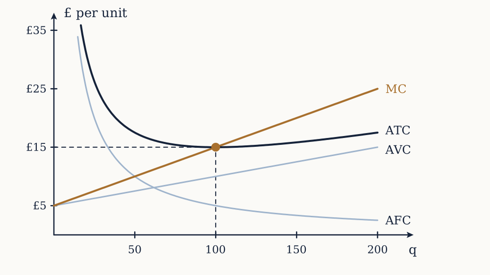
So average total cost falls while marginal cost is below it, rises while marginal is above it, and is stationary where they are equal. Marginal cost cuts average total cost at the minimum of average cost, and it does so from below. The same argument applies to average variable cost. This is not an empirical regularity or a drawing convention; it is a consequence of what an average is, and it will be doing serious work in the next two lessons.

Example. A firm has $C (q) = 500 + 5 q + 0.05 q^{2}$ . Find the four cost measures at $q = 50$ , $q = 100$ and $q = 150$ , and locate the minimum of average total cost.

Marginal cost is $MC = 5 + 0.1 q$ . At $q = 50$ : total cost is $500 + 250 + 125 = £ 875$ , so $AFC = 10$ , $AVC = 7.50$ , $ATC = 17.50$ , and $MC = £ 10$ . Marginal is below average, so average is falling. At $q = 100$ : total cost is £1500, $ATC = £ 15$ , and $MC = £ 15$ . They are equal, so this is the minimum. At $q = 150$ : total cost is £2375, $ATC = £ 15.83$ , and $MC = £ 20$ ; marginal is above average and average is climbing again. Confirming by calculus: $ATC = 500 / q + 5 + 0.05 q$ , and setting the derivative $- 500 / q^{2} + 0.05$ to zero gives $q^{2} = 10000$ , so $q = 100$ .

Now you. A firm has $C (q) = 800 + 4 q + 0.02 q^{2}$ . Find the output that minimises average total cost, and the value of average and marginal cost there.

Answer

$ATC = 800 / q + 4 + 0.02 q$ , and $- 800 / q^{2} + 0.02 = 0$ gives $q^{2} = 40000$ , so $q = 200$ . There $ATC = 4 + 4 + 4 = £ 12$ and $MC = 4 + 0.04 (200) = £ 12$ . They agree, as they must at the minimum.

One honest note about this example. Its average variable cost, $5 + 0.05 q$ , rises from the very first unit, so it has no U-shape. A U-shaped average variable cost requires a range over which marginal product is rising, which needs a cubic variable cost rather than a quadratic one. Textbook diagrams almost always draw the U; a great many real short-run cost functions look more like this one, with marginal cost roughly flat over normal operating ranges and turning up sharply near capacity.

The long run is an envelope

In the long run nothing is fixed, so the firm picks the plant as well as the output. Suppose it can build any of a family of plants, each with its own short-run cost curve. For any output it will use the plant that makes that output most cheaply, so the long-run average cost curve is the lower envelope of all the short-run curves: at each output it takes the smallest value any plant offers.

Two consequences follow. Long-run average cost is never above short-run average cost at the same output, because building the right plant is always an option. And the envelope touches each short-run curve at exactly one output, the one that plant is optimal for, which need not be that plant's own cheapest output.

Example. A firm can build a small plant with $C_{1} = 500 + 0.05 q^{2}$ or a medium one with $C_{2} = 2000 + 0.0125 q^{2}$ . At what output should it switch, and what is average cost on either side?

Setting the totals equal: $500 + 0.05 q^{2} = 2000 + 0.0125 q^{2}$ , so $0.0375 q^{2} = 1500$ and $q = 200$ . At $q = 100$ the small plant gives average cost $1000 / 100 = £ 10$ against the medium plant's $2125 / 100 = £ 21.25$ , so small wins. At $q = 400$ the small plant gives £21.25 and the medium gives £10, so medium wins. At the switch point both cost £2500, an average of £12.50 each.

Now you. A large plant costs $C_{3} = 8000 + 0.003125 q^{2}$ . At what output does the firm switch from the medium plant to the large one?

Answer

$2000 + 0.0125 q^{2} = 8000 + 0.003125 q^{2}$ gives $0.009375 q^{2} = 6000$ , so $q^{2} = 640000$ and $q = 800$ . Both plants then cost £10,000, an average of £12.50. Each plant's own cheapest output is 100, 400 and 1600 respectively, and at each of those the average cost is exactly £10, so the long-run average cost curve here is flat at £10 and touches each short-run curve at its own minimum. That coincidence only happens when long-run average cost is constant.

Economies of scale, and how far they go

Long-run average cost falling with output is economies of scale; rising is diseconomies. The sources of the first were listed in the previous lesson: indivisibilities, specialisation, and the geometric fact that container volume grows faster than container surface. Diseconomies are mostly about management. Coordination, monitoring and information loss grow more than proportionally with the number of people who have to agree on something, and no technology has abolished that.

The scale at which average cost stops falling is the minimum efficient scale, and it is the single most useful number about an industry, because it sets how many firms the market can hold. A market whose total demand is ten times the minimum efficient scale can support ten efficient firms; one whose demand is twice it cannot support more than two. Structure follows from technology, which is why the market structure lessons come after this one rather than before.

The measured picture is less dramatic than the textbook diagram. Laurits Christensen and William Greene, studying United States electricity generation in 1976, found that scale economies had largely been exhausted by 1970, with most output produced by firms already operating on the flat part of the curve. Car assembly is usually put in the low hundreds of thousands of vehicles a year per plant, well below world demand, which is why the industry has many producers rather than one. Long-run average cost curves in practice tend to be L-shaped: falling sharply, then flat over a wide range, rather than U-shaped with a single sweet spot.

Cost falls with experience, not only with scale

One effect the whole apparatus of this lesson misses is that costs fall over time with cumulative production, independently of the current rate of output. T. P. Wright measured it on airframes in 1936 and found that each doubling of cumulative units built cut labour cost per unit by roughly 20 per cent. The same pattern has since been documented across semiconductors, wind turbines and photovoltaic modules, where the learning rate is also around 20 per cent per doubling and has held over more than four orders of magnitude of cumulative output.

This is a different axis from scale. Economies of scale are about output per year; learning is about output ever. A firm can sit at the same annual rate for a decade and still see its costs fall. Nothing in a static cost function represents this, and any argument about industrial policy that turns on infant industries is really an argument about learning curves rather than about scale.

The firm now has a cost function and knows what any output would cost. It still has no reason to pick one output rather than another, because nothing has yet been said about what the output sells for. Supplying that is the next lesson, and the answer depends entirely on how much market power the firm has.