Vectors

A column of numbers can be read as an arrow in space, and the two readings support exactly the same arithmetic, which is what makes the geometry of the previous lesson available to systems of any size.

The previous lesson ended by writing a system of three equations as a statement about three columns of coefficients, $x (2, - 3, - 2) + y (1, - 1, 1) + z (- 1, 2, 2) = (8, - 11, - 3)$ . Two things happened to those columns there: they were multiplied by numbers, and they were added. This lesson takes those two operations as the definition of the objects, and then shows that measurement, length and angle and perpendicularity, comes from one further product that is not part of the definition at all.

An arrow and a list

A vector in the plane can be pictured as an arrow with a length and a direction, and represented by the pair of numbers saying how far it goes across and how far up: $(3, 4)$ is three to the right and four up. The arrow is not anchored anywhere. An arrow from $(1, 1)$ to $(4, 5)$ and an arrow from the origin to $(3, 4)$ are the same vector, because both are three across and four up, and it is convenient to draw every vector from the origin so that vectors and points can be identified.

In three dimensions the same works with triples, and beyond three the picture stops but the arithmetic does not. A vector in $R^{n}$ is an ordered list of $n$ real numbers, and $n$ can be a million. This is not an abstraction for its own sake. A greyscale image of 1000 by 1000 pixels is a vector in $R^{1000000}$ , one coordinate per pixel. A month of daily closing prices for thirty stocks is a vector in $R^{900}$ . The word "direction" is unvisualisable in those spaces and remains perfectly well defined.

Two vectors are equal when every component matches. The zero vector $0$ has every component zero, and it is the one vector with no direction. Vectors are written in bold, $v$ , and their components with subscripts, so $v = (v_{1}, v_{2}, \dots, v_{n})$ . Throughout this course a vector written in round brackets is a column, which matters from the lesson on matrices onward.

Two operations, and only two

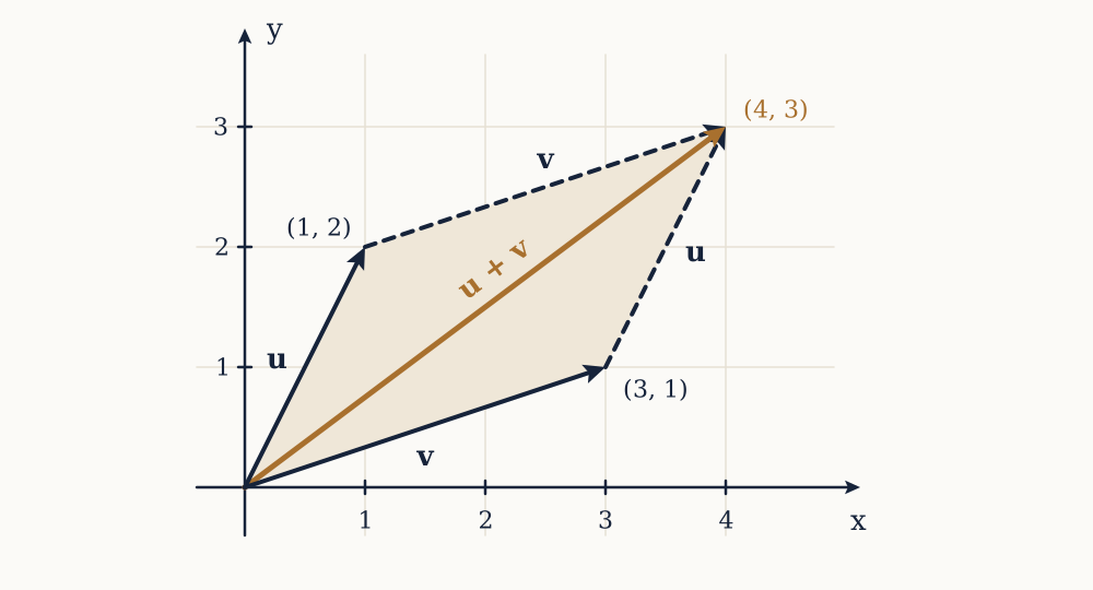
Addition works component by component: $(1, 2) + (3, 1) = (4, 3)$ . Geometrically it is tip to tail. Draw the first arrow, start the second where the first ended, and the sum runs from the original start to the final tip. Equivalently, complete the parallelogram with the two arrows as sides and take its diagonal. That the two constructions agree is the statement that $u + v = v + u$ , which is obvious from the components and not obvious from the picture.

Scalar multiplication multiplies every component by a number: $2 (1, 2) = (2, 4)$ and $- 0.5 (4, 3) = (- 2, - 1.5)$ . The number is called a scalar to distinguish it from a vector. Geometrically, multiplying by $c$ stretches the arrow by a factor $| c |$ , and reverses it when $c$ is negative. All the scalar multiples of one non-zero vector, taken together, form an infinite straight line through the origin.

Subtraction is not a third operation, being $u + (- 1) v$ , and it is worth reading geometrically: $u - v$ is the arrow from the tip of $v$ to the tip of $u$ . That reading is used constantly, because the vector between two points is the difference of their position vectors.

There is deliberately no multiplication of two vectors in this list, and no division at all. The reason is that the operations are chosen to be exactly those that a system of linear equations performs, and the definition is worth stating in that spirit: a vector space is any set on which addition and scalar multiplication are defined and obey eight rules, that addition is commutative and associative, that a zero exists and each element has a negative, that scaling distributes over both kinds of sum, that $(c d) v = c (d v)$ , and that $1 v = v$ . Lists of $n$ numbers satisfy them. So do polynomials of degree at most five, which can be added and scaled and form a space of a size worked out two lessons from now. So do all real-valued functions on an interval, and so do the solutions of a differential equation like $y^{''} + y = 0$ . Every result in this course rests on the eight rules alone, so every result applies to all of those, which is the return on the abstraction.

Example. With $u = (2, - 1, 3)$ and $v = (1, 4, - 2)$ , compute $3 u - 2 v$ .

Scale first: $3 u = (6, - 3, 9)$ and $2 v = (2, 8, - 4)$ . Subtract component by component: $(6 - 2, - 3 - 8, 9 + 4) = (4, - 11, 13)$ .

Now you. With the same $u$ and $v$ , compute $u + 2 v$ and check that it equals $(4, 7, - 1)$ .

Answer

$2 v = (2, 8, - 4)$ , so $u + 2 v = (2 + 2, - 1 + 8, 3 - 4) = (4, 7, - 1)$ . The check is componentwise, and each one has to work independently.

Length

Nothing said so far measures anything. Length has to be added, and in the plane Pythagoras supplies it: the arrow $(3, 4)$ is the hypotenuse of a right triangle with legs $3$ and $4$ , so its length is $\sqrt{9 + 16} = 5$ . In three dimensions apply Pythagoras twice, once in the base plane and once vertically, giving $\sqrt{v_{1}^{2} + v_{2}^{2} + v_{3}^{2}}$ . The vector $(1, 2, 2)$ has length $\sqrt{1 + 4 + 4} = 3$ exactly.

In $n$ dimensions the same formula is taken as the definition, since there is no triangle to appeal to:

‖ v ‖ = \sqrt{v_{1}^{2} + v_{2}^{2} + \dots + v_{n}^{2}}

The double bars distinguish it from the absolute value of a number, which it generalises. Length is never negative, and is zero only for the zero vector. Scaling behaves as the picture demands: $‖ c v ‖ = | c | ‖ v ‖$ , because every component is multiplied by $c$ and every square by $c^{2}$ .

A vector of length one is a unit vector, and dividing any non-zero vector by its own length produces one pointing the same way, an operation called normalising. This separates a vector into a direction and a magnitude, which is what makes it useful.

Example. Find the length of $(5, - 12)$ and the unit vector in its direction.

$‖ (5, - 12) ‖ = \sqrt{25 + 144} = \sqrt{169} = 13$ . Dividing gives $(5 / 13, - 12 / 13) = (0.3846, - 0.9231)$ , and as a check ${0.3846}^{2} + {0.9231}^{2} = 0.1479 + 0.8521 = 1.0000$ .

Now you. Find the length of $(2, 3, 6)$ and normalise it.

Answer

$\sqrt{4 + 9 + 36} = \sqrt{49} = 7$ , so the unit vector is $(2 / 7, 3 / 7, 6 / 7) = (0.2857, 0.4286, 0.8571)$ . Squaring and adding gives $0.0816 + 0.1837 + 0.7347 = 1.0000$ .

The dot product

Angles need one more construction, and it is the single most useful formula in the subject. The dot product of two vectors with the same number of components multiplies them componentwise and adds the results:

a \cdot b = a_{1} b_{1} + a_{2} b_{2} + \dots + a_{n} b_{n}

The output is a number, not a vector, which is why it is also called the scalar product. For $(1, 2)$ and $(3, 1)$ it is $3 + 2 = 5$ . It is commutative, it distributes over addition, and it relates to length by $a \cdot a = ‖ a ‖^{2}$ , straight from the definitions.

Its geometric meaning is not visible in that formula and has to be derived. Take two vectors $a$ and $b$ with angle $θ$ between them. The three arrows $a$ , $b$ and $b - a$ form a triangle, so the law of cosines from Mathematical Foundations gives

‖ b - a ‖^{2} = ‖ a ‖^{2} + ‖ b ‖^{2} - 2 ‖ a ‖ ‖ b ‖ \cos θ

Now expand the left side algebraically instead. Since $‖ b - a ‖^{2} = (b - a) \cdot (b - a)$ , distributing gives $b \cdot b - 2 a \cdot b + a \cdot a$ , which is $‖ b ‖^{2} - 2 a \cdot b + ‖ a ‖^{2}$ . Setting the two expressions equal, the squared lengths cancel from both sides and what remains is

a \cdot b = ‖ a ‖ ‖ b ‖ \cos θ

So a formula built out of nothing but multiplication and addition of coordinates knows the angle. Rearranged, $\cos θ = a \cdot b / (‖ a ‖ ‖ b ‖)$ , and this is taken as the definition of angle in dimensions too high to draw.

One consequence deserves its own name. Since $\cos 90 ° = 0$ , two non-zero vectors are orthogonal, meaning perpendicular, exactly when their dot product is zero. Checking perpendicularity is therefore a multiplication and an addition, with no trigonometry and no picture. Almost everything later in this course that involves a right angle is really this test being applied.

A second consequence is that $| \cos θ | \leq 1$ forces $| a \cdot b | \leq ‖ a ‖ ‖ b ‖$ , the Cauchy-Schwarz inequality, holding in every dimension. For $(1, 2)$ and $(3, 1)$ it reads $5 \leq \sqrt{5} \sqrt{10} = 7.071$ , with equality only when the vectors are parallel.

Example. Find the angle between $(1, 2)$ and $(3, 1)$ .

The dot product is $1 (3) + 2 (1) = 5$ . The lengths are $\sqrt{5} = 2.2361$ and $\sqrt{10} = 3.1623$ , whose product is $\sqrt{50} = 7.0711$ . So $\cos θ = 5 / 7.0711 = 0.70711$ , and $θ = 45 °$ exactly, since $\cos 45 ° = 1 / \sqrt{2}$ .

Now you. Find the angle between $(2, - 1)$ and $(1, 3)$ .

Answer

The dot product is $2 - 3 = - 1$ , and the lengths are again $\sqrt{5}$ and $\sqrt{10}$ , so $\cos θ = - 1 / 7.0711 = - 0.14142$ and $θ = 98.13 °$ . The negative dot product is the signal that the angle is obtuse, which is worth recognising without computing the arccosine.

What the dot product measures

Physics fixed the meaning before linear algebra did. Work is force times distance only when the two point the same way, and in general the work done by a constant force $F$ through a displacement $d$ is $F \cdot d$ . Take a force $(12, 5)$ newtons dragging an object through a displacement $(3, 4)$ metres. The dot product is $36 + 20 = 56$ joules. Checking against the other formula: the force has magnitude $13$ N, the displacement $5$ m, and the angle between them is $30.51 °$ , so $13 \times 5 \times \cos 30.51 ° = 65 \times 0.8615 = 56$ J. The two routes agree, as the derivation says they must, and the second one shows what is happening: only the part of the force lying along the displacement does any work.

That reading, how much of one vector lies along another, is what the dot product measures. If $u$ is a unit vector then $a \cdot u$ is exactly the length of the shadow $a$ casts on $u$ 's line, signed so that a shadow falling the other way counts negative. Take $a = (4, 3)$ and $u = (1, 0)$ : the dot product is $4$ , which is the $x$ coordinate, which is the shadow on the horizontal axis. Coordinates are dot products with the axis directions, a fact that looks like a triviality here and becomes a labour-saving device in the lesson on orthogonality.

Projection

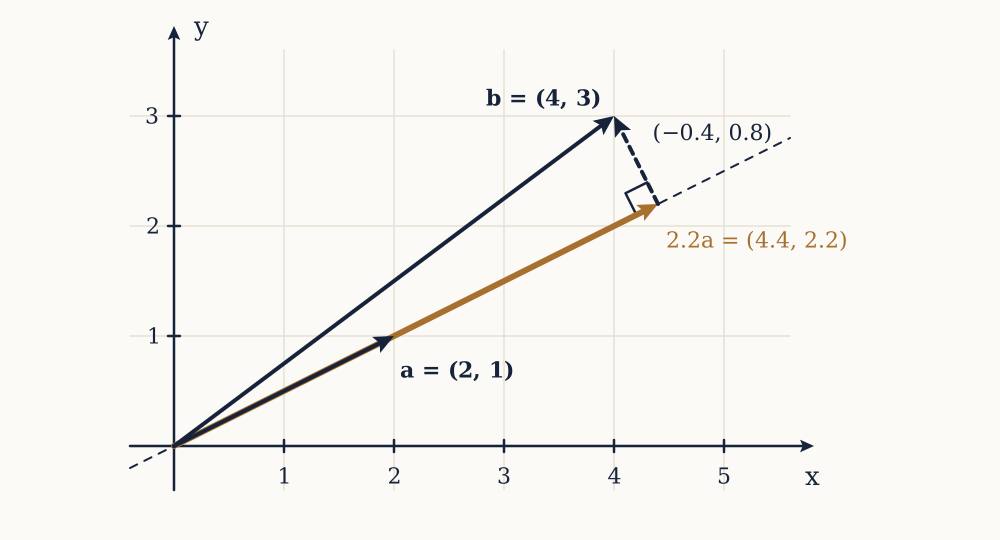
Make that precise for a general direction. Given $b$ and a non-zero $a$ , the projection of $b$ onto $a$ is the multiple of $a$ that lies directly under $b$ , meaning the multiple $c a$ for which the leftover $b - c a$ is perpendicular to $a$ . That one condition determines $c$ : orthogonality means $a \cdot (b - c a) = 0$ , so $a \cdot b = c a \cdot a$ and

c = \frac{a \cdot b}{a \cdot a}

with the projection itself being $c a$ . Nothing was assumed about the dimension, so this works in $R^{900}$ as readily as in the plane.

The projection splits $b$ into two pieces, one along $a$ and one perpendicular to it, and that decomposition is used everywhere from resolving forces on a slope to the least squares fitting three lessons ahead.

Example. Project $b = (4, 3)$ onto $a = (2, 1)$ , and split $b$ into parallel and perpendicular parts.

$a \cdot b = 8 + 3 = 11$ and $a \cdot a = 4 + 1 = 5$ , so $c = 2.2$ and the projection is $2.2 (2, 1) = (4.4, 2.2)$ . The leftover is $(4 - 4.4, 3 - 2.2) = (- 0.4, 0.8)$ , and its dot product with $a$ is $- 0.8 + 0.8 = 0$ , confirming the right angle. The two pieces sum back to $(4, 3)$ .

Now you. Project $b = (5, 2)$ onto $a = (1, 3)$ and check the leftover is perpendicular.

Answer

$a \cdot b = 5 + 6 = 11$ and $a \cdot a = 1 + 9 = 10$ , so $c = 1.1$ and the projection is $(1.1, 3.3)$ . The leftover is $(3.9, - 1.3)$ , whose dot product with $(1, 3)$ is $3.9 - 3.9 = 0$ .

Honest limits

The dot product formula $a_{1} b_{1} + \dots + a_{n} b_{n}$ is not a property of the vectors alone: it assumes the coordinates are measured along axes that are themselves perpendicular and equally scaled. Write the same arrows in a slanted coordinate system and the componentwise formula stops giving the right angles. The lesson on change of basis returns to this, and orthogonal bases matter later precisely because they are the ones where the easy formula stays true.

Two other cautions. The cross product, which takes two vectors to a third, exists only in three dimensions and is not part of this course. And the dot product of two vectors of the same length is a poor measure of similarity when the vectors have very different magnitudes, which is why applied work usually normalises first and compares $\cos θ$ rather than the raw product.

Addition and scaling are now the whole toolkit, and length and angle sit on top of them. Applying those two operations to a fixed collection of vectors, over and over, generates everything the collection can reach, and the next lesson asks what that reachable set looks like and when one of the vectors in the collection is contributing nothing.