Linear transformations

Everything so far has sat still, and the subject only becomes useful when something moves the vectors around.

The previous lessons built the objects: vectors, added and scaled, spanning subspaces that have a dimension and a basis. Nothing in them acts. This lesson introduces maps from one space to another, restricts them to the ones that respect the two operations, and finds that the restriction is so severe that such a map can be written down completely with a handful of numbers.

The definition, and what it rules out

A map $T$ from $R^{n}$ to $R^{m}$ is linear when it satisfies two conditions for all vectors $u, v$ and all scalars $c$ :

T (u + v) = T (u) + T (v) T (c v) = c T (v)

In words: it does not matter whether you add before or after applying $T$ , and it does not matter whether you scale before or after. The two together say $T$ preserves linear combinations, $T (a u + b v) = a T (u) + b T (v)$ , which is the form actually used in proofs.

An immediate consequence is $T (0) = 0$ : take $c = 0$ in the second condition. A linear map cannot move the origin, and that alone rules out a large class of familiar operations.

Translation is the important casualty. The map $T (x, y) = (x + 1, y)$ , sliding the plane one unit right, is not linear, because $T (0, 0) = (1, 0) \neq 0$ . This is not a technicality to be regretted: translations are excluded on purpose, because including them would destroy the theory, and the practical fix is the affine trick mentioned at the end of this lesson.

Squaring fails too. For $T (x, y) = (x^{2}, y)$ , compare $T (2, 0) = (4, 0)$ with $2 T (1, 0) = (2, 0)$ . Scaling the input doubled the output in one place and quadrupled it in another, so the second condition fails. And a map can satisfy one condition while failing the other, so both must be checked.

What survives is a smaller class than intuition suggests, and it contains exactly the operations that stretch, rotate, reflect, shear, project and collapse, applied uniformly to the whole space. Geometrically, a linear map on the plane sends straight lines to straight lines, keeps the origin fixed, and sends a grid of parallel evenly spaced lines to another grid of parallel evenly spaced lines, though the grid may be tilted, stretched or flattened.

Example. Is $T (x, y) = (2 x - y, x + 3 y)$ linear?

Take $u = (u_{1}, u_{2})$ and $v = (v_{1}, v_{2})$ . Then $T (u + v) = (2 (u_{1} + v_{1}) - (u_{2} + v_{2}), (u_{1} + v_{1}) + 3 (u_{2} + v_{2}))$ , and expanding and regrouping gives $(2 u_{1} - u_{2}, u_{1} + 3 u_{2}) + (2 v_{1} - v_{2}, v_{1} + 3 v_{2}) = T (u) + T (v)$ . Scaling works the same way, since every term carries exactly one factor of an input component. So it is linear, and the general rule is visible: a map whose output components are sums of the input components multiplied by constants, with no constant term, is linear.

Now you. Is $T (x, y) = (x + y, x y)$ linear?

Answer

No. $T (2, 0) = (2, 0)$ and $T (0, 2) = (2, 0)$ , so the sum of the outputs is $(4, 0)$ , while $T (2, 2) = (4, 4)$ . Addition is not preserved. The second component multiplies two input components together, which is exactly what linearity forbids.

A map is fixed by what it does to a basis

Here is the theorem that makes the subject computational. Write any vector in the plane in the standard basis, $v = (x, y) = x e_{1} + y e_{2}$ where $e_{1} = (1, 0)$ and $e_{2} = (0, 1)$ . Applying a linear $T$ and using both conditions,

T (v) = T (x e_{1} + y e_{2}) = x T (e_{1}) + y T (e_{2})

The right hand side involves $T$ only at the two basis vectors. So if you know where $T$ sends $e_{1}$ and where it sends $e_{2}$ , you know where it sends everything, with no further information required. In $R^{n}$ the same argument uses $n$ basis vectors, and in any subspace it uses a basis of that subspace.

This is a strong statement. A general function from the plane to the plane requires specifying two numbers for each of infinitely many points. A linear one requires four numbers in total.

Suppose $T (e_{1}) = (3, 1)$ and $T (e_{2}) = (- 1, 2)$ . Then $T (4, 5) = 4 (3, 1) + 5 (- 1, 2) = (12 - 5, 4 + 10) = (7, 14)$ , and every other value of $T$ is available the same way.

The matrix of a transformation

Record those images as the columns of an array, and the array is the matrix of $T$ . Following the convention fixed in the first lesson, a matrix is written as the list of its columns, so the map above has matrix

A = [(3, 1), (- 1, 2)]

whose first column is $T (e_{1})$ and whose second is $T (e_{2})$ . This is the single most useful sentence in the subject: the columns of a matrix are the images of the basis vectors. Read a matrix that way and its geometry is visible without any computation.

The product $A x$ is then defined to be exactly what the theorem says $T (x)$ is:

A x = x_{1} (column 1) + x_{2} (column 2) + \dots

a linear combination of the columns with the components of $x$ as the weights. Taking $A = [(2, 1), (- 1, 3)]$ and $x = (4, 2)$ : $4 (2, 1) + 2 (- 1, 3) = (8 - 2, 4 + 6) = (6, 10)$ .

The same number can be computed the other way round, taking one output component at a time: the $i$ th component of $A x$ is the $i$ th row of $A$ dotted with $x$ . Here the first row is $(2, - 1)$ , giving $8 - 2 = 6$ , and the second row is $(1, 3)$ , giving $4 + 6 = 10$ . The row method is how the arithmetic is usually organised, and the column method is what it means. Both give the same answer, because both are the same sum of products with the terms gathered differently.

An $m$ by $n$ matrix has $n$ columns, each of length $m$ , and represents a map from $R^{n}$ to $R^{m}$ : it eats vectors with $n$ components and produces vectors with $m$ . Note the order, which trips everyone at first: the number of columns is the dimension of the input space.

With this, the very first lesson's system becomes $A x = b$ , and the whole subject is one notation. Solving a system asks which input $A$ sends to a given output.

Example. A linear map doubles every vector and then rotates it a quarter turn anticlockwise. What is its matrix?

Follow the basis vectors. $e_{1} = (1, 0)$ doubles to $(2, 0)$ , and a quarter turn anticlockwise sends it to $(0, 2)$ . $e_{2} = (0, 1)$ doubles to $(0, 2)$ , and turning sends it to $(- 2, 0)$ . So the matrix is $[(0, 2), (- 2, 0)]$ . Test it on $(3, 1)$ : the formula gives $3 (0, 2) + 1 (- 2, 0) = (- 2, 6)$ , and by hand, doubling gives $(6, 2)$ and a quarter turn sends $(6, 2)$ to $(- 2, 6)$ .

Now you. A linear map reflects in the horizontal axis and then multiplies every length by three. What is its matrix?

Answer

$e_{1} = (1, 0)$ is unmoved by the reflection and becomes $(3, 0)$ . $e_{2} = (0, 1)$ reflects to $(0, - 1)$ and becomes $(0, - 3)$ . The matrix is $[(3, 0), (0, - 3)]$ . Applied to $(2, 5)$ it gives $2 (3, 0) + 5 (0, - 3) = (6, - 15)$ , which is the reflection $(2, - 5)$ tripled.

A catalogue of plane transformations

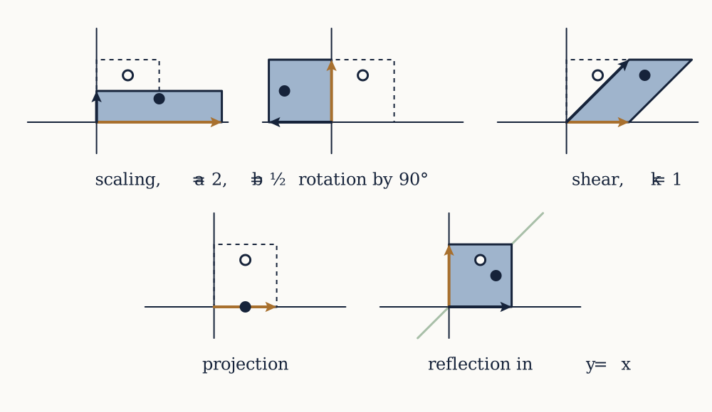
Every entry below is obtained the same way, by asking where $e_{1}$ and $e_{2}$ go. None of them needs to be memorised.

Scaling. Stretching by $a$ horizontally and $b$ vertically sends $e_{1}$ to $(a, 0)$ and $e_{2}$ to $(0, b)$ , giving $[(a, 0), (0, b)]$ . With $a = b$ this is a uniform scaling, and with $a = b = 1$ it is the identity matrix $I = [(1, 0), (0, 1)]$ , which leaves every vector alone.

Rotation. Turn the plane anticlockwise by $θ$ . The vector $e_{1}$ lands on the unit circle at angle $θ$ , which is $(\cos θ, \sin θ)$ . The vector $e_{2}$ starts a quarter turn ahead of $e_{1}$ and stays a quarter turn ahead, landing at angle $θ + 90 °$ , which is $(- \sin θ, \cos θ)$ . So

R_{θ} = [(\cos θ, \sin θ), (- \sin θ, \cos θ)]

For $θ = 90 °$ this is $[(0, 1), (- 1, 0)]$ , matching the quarter turn used above. That entire derivation is two sentences of trigonometry, which is why the rotation matrix is worth deriving rather than remembering.

Shear. Fix the horizontal axis and slide everything else sideways in proportion to its height: $e_{1}$ stays at $(1, 0)$ and $e_{2}$ moves to $(k, 1)$ . The matrix is $[(1, 0), (k, 1)]$ . With $k = 1$ the point $(2, 3)$ goes to $2 (1, 0) + 3 (1, 1) = (5, 3)$ : the height is unchanged and the horizontal displacement equals the height. This is what italic type does to letters.

Projection. Flatten the plane onto the horizontal axis: $e_{1}$ stays and $e_{2}$ goes to $0$ , giving $[(1, 0), (0, 0)]$ . Information is destroyed here, since every point with the same $x$ has the same image, and that irreversibility is the subject of two lessons from now.

Reflection. Reflecting in the line $y = x$ swaps the axes, so $e_{1} \mapsto (0, 1)$ and $e_{2} \mapsto (1, 0)$ , giving $[(0, 1), (1, 0)]$ . For a general line through the origin at angle $θ$ , reflecting sends $e_{1}$ to angle $2 θ$ and $e_{2}$ to angle $2 θ - 90 °$ , giving $[(\cos 2 θ, \sin 2 θ), (\sin 2 θ, - \cos 2 θ)]$ . Setting $θ = 45 °$ recovers the swap, since $\cos 90 ° = 0$ and $\sin 90 ° = 1$ .

Example. Rotate $(2, 0)$ by $30 °$ and confirm the length is unchanged.

The matrix is $[(\cos 30 °, \sin 30 °), (- \sin 30 °, \cos 30 °)] = [(0.8660, 0.5000), (- 0.5000, 0.8660)]$ . Applying it, $2 (0.8660, 0.5000) + 0 (\dots) = (1.7321, 1.0000)$ . The length is $\sqrt{3 + 1} = 2$ , unchanged, as a rotation demands. The exact answer is $(\sqrt{3}, 1)$ .

Now you. Rotate $(0, 3)$ by $60 °$ .

Answer

Only the second column contributes: $3 (- \sin 60 °, \cos 60 °) = 3 (- 0.8660, 0.5000) = (- 2.598, 1.500)$ . The length is $\sqrt{6.750 + 2.250} = \sqrt{9} = 3$ , unchanged. The exact answer is $(- 3 \sqrt{3} / 2, 3 / 2)$ .

Why the restriction pays

Linearity is what makes a transformation knowable from finitely many measurements, and the consequences run further than convenience.

Because $T$ preserves combinations, it maps subspaces to subspaces: the image of a line through the origin is a line through the origin or the single point $0$ , and the image of a plane is a plane, a line or a point. Nothing bends, and nothing that was flat becomes curved.

Because $T$ is determined on a basis, two maps agreeing on a basis are the same map everywhere, which is the standard way of proving that two matrices are equal. And because the matrix is just a list of images, building a transformation to specification is a matter of writing down where you want the basis to go, which is how every rotation in a graphics engine and every filter in signal processing is constructed.

The catalogue also shows what to watch for. Rotations and reflections preserve length; scalings and shears do not; projections destroy information. Those distinctions get numbers attached to them in the next three lessons.

Honest limits

Translation is not linear, and yet moving objects around is most of what computer graphics does. The standard fix is to embed the plane in three dimensions as the slice $z = 1$ , where a translation of the plane becomes a shear of the larger space, which is linear. Points then carry an extra coordinate, called homogeneous coordinates, and this is why graphics hardware works with four by four matrices for three-dimensional scenes: three dimensions of geometry plus one for the trick. Maps of the form $T (x) = A x + b$ are called affine, and they are the ones that preserve straight lines without fixing the origin.

Second, the matrix of a map depends on the basis used to write it down. Everything above used the standard basis silently. The same transformation gets a different matrix in a different basis, and choosing a basis that makes the matrix simple is the whole strategy of the last third of this course.

Third, real data is rarely linear, and calling a model linear is a claim that can be wrong. Doubling the dose does not always double the effect. The usual defence is that a smooth relationship is approximately linear over a small enough range, which is exactly what a derivative asserts, and the approximation fails outside that range without any warning from the algebra.

One transformation is now four numbers. Two transformations applied in turn are also a transformation, so it too has four numbers, and asking how to compute them from the original eight is what defines matrix multiplication in the next lesson.