Lagrange multipliers

A firm maximising output cannot choose any labour and capital it likes, because it has a budget, and the best point on the budget line is almost never a point where the gradient of output vanishes.

The previous lesson found maxima and minima by setting the gradient $\nabla f$ to zero and sorting the critical points with the second derivative test. It ended on the catch: real problems restrict the inputs to a curve or a surface (a fixed amount of material, a budget, a plane to stay on), and the best point there can sit on a steep hillside of $f$ . It assumes the gradient and the fact, proved in an earlier lesson, that $\nabla g$ is perpendicular to the level curve of $g$ through the point.

Substituting the constraint

The obvious approach is to use the constraint to eliminate a variable. A farmer with $200$ metres of fencing encloses a rectangle of sides $x$ and $y$ , so $2 x + 2 y = 200$ , and wants the area $x y$ as large as possible. Solving the constraint gives $y = 100 - x$ , the area becomes $A (x) = 100 x - x^{2}$ on $0 \leq x \leq 100$ , and $A^{'} (x) = 100 - 2 x = 0$ at $x = 50$ . The best field is a square of $2500$ square metres.

It fails quietly as soon as the constraint is less tidy. Take $f (x, y) = x^{2} + y^{2}$ , the squared distance from the origin, on the ellipse $\frac{x^{2}}{4} + y^{2} = 1$ . Substituting $y^{2} = 1 - \frac{x^{2}}{4}$ gives $f = 1 + \frac{3 x^{2}}{4}$ , whose derivative $\frac{3 x}{2}$ vanishes only at $x = 0$ , where $f = 1$ . That is the minimum. The maximum, $f = 4$ at $(\pm 2, 0)$ , is missed entirely: it sits at the ends of the interval $- 2 \leq x \leq 2$ on which the substitution is valid, a restriction the formula $1 + \frac{3 x^{2}}{4}$ does not remember.

Other constraints cannot be solved at all: the closed curve $x^{4} + y^{4} + x y = 3$ needs a quartic solved for $y$ . What is wanted is a method that takes the constraint as a level set $g (x, y) = c$ and never solves it.

Where a contour touches the constraint

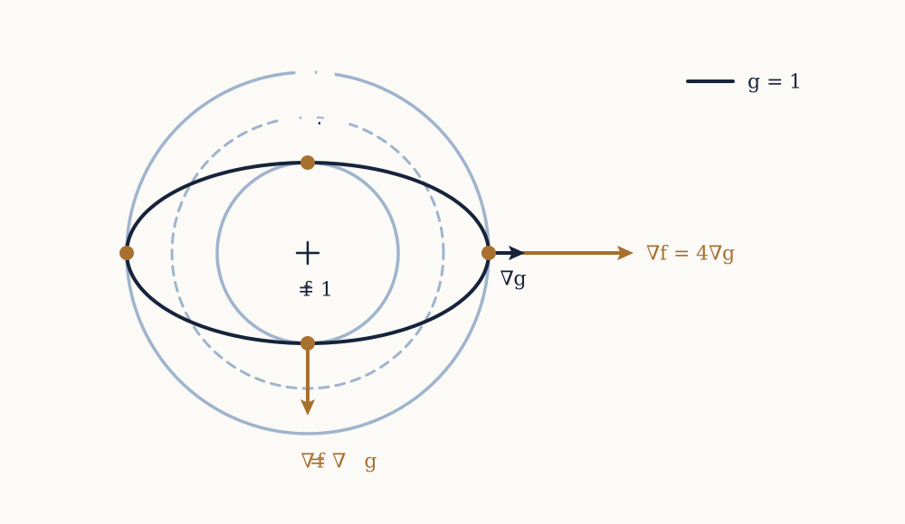
Lay the constraint curve $g (x, y) = c$ over the contour map of $f$ and walk along it. Where the constraint cuts a contour at an angle, $f$ is higher on one side of the crossing and lower on the other, so that point is neither a maximum nor a minimum along the walk. The only places the walk can turn round in $f$ are where the constraint does not cut the contour but grazes it: at a constrained extremum the level curve of $f$ is tangent to the constraint curve.

The chain rule makes this exact. Let $𝐫 (t) = (x (t), y (t))$ trace the constraint curve, passing the point $P$ at $t = 0$ with velocity $𝐯 \neq 𝟎$ . If $f$ restricted to the curve is extreme at $P$ , the single variable function $f (𝐫 (t))$ is extreme at $t = 0$ , so its derivative vanishes, and by the chain rule along a path

\nabla f (P) \cdot 𝐯 = 0

So $\nabla f$ is perpendicular to the constraint at $P$ . So is $\nabla g$ , since $g (𝐫 (t)) = c$ for every $t$ and differentiating gives $\nabla g (P) \cdot 𝐯 = 0$ . In the plane, two vectors perpendicular to the same nonzero direction lie on one line. Provided $\nabla g (P) \neq 𝟎$ , there is therefore a number $λ$ with

\nabla f (P) = λ \nabla g (P)

This is the tangency of the picture restated: the gradients are the normals of the two curves, and parallel normals mean the curves share a tangent line. The number $λ$ , the Greek letter lambda, is called a Lagrange multiplier, after Joseph-Louis Lagrange, who used it in his Mécanique analytique of 1788 for mechanical systems held by constraints. It can be positive, negative or zero.

On a constraint surface $g (x, y, z) = c$ the same argument applies to every curve through $P$ , so $\nabla f (P)$ is perpendicular to the whole tangent plane, as is its normal $\nabla g (P)$ . Again $\nabla f = λ \nabla g$ .

The method

Written out in components, $\nabla f = λ \nabla g$ together with the constraint is a system of equations:

f_{x} = λ g_{x}, f_{y} = λ g_{y}, g (x, y) = c

That is three equations in the three unknowns $x$ , $y$ and $λ$ , or four in four with $z$ . Solve it, evaluate $f$ at every solution, and compare. The solutions are candidates, like the critical points of the previous lesson, not answers. When the constraint set is closed and bounded, such as an ellipse or a sphere, a continuous $f$ is guaranteed a largest and a smallest value on it, and they are among the candidates (together with any points where $\nabla g = 𝟎$ , which the argument above excluded). When the set is unbounded, a separate argument is needed that an extremum exists at all.

The ellipse that defeated substitution shows the method at work. With $f = x^{2} + y^{2}$ and $g = \frac{x^{2}}{4} + y^{2} = 1$ , the equations are $2 x = λ \frac{x}{2}$ and $2 y = 2 λ y$ . The first says $x = 0$ or $λ = 4$ ; the second says $y = 0$ or $λ = 1$ . Taking $x = 0$ , the constraint gives $y = \pm 1$ and $f = 1$ . Taking $λ = 4$ , the second equation forces $y = 0$ , so $x = \pm 2$ and $f = 4$ . Both the minimum and the missed maximum appear, and at each the ellipse touches a circle centred on the origin, the level curves of $f$ .

The ellipse x²/4 + y² = 1 with level circles of f = x² + y². It touches the circle f = 1 at (0, ±1), the minimum, and the circle f = 4 at (±2, 0), the maximum, while the dashed circle f = 2.25 cuts straight across it. At the touching points the gradients line up: ∇f = ∇g at (0, −1), where λ = 1, and ∇f = 4∇g at (2, 0), where λ = 4.

Example. An open-topped box is to be made from $12$ square metres of sheet metal. What dimensions give the largest volume?

With base $x$ by $y$ and height $z$ , maximise $V = x y z$ subject to $g = x y + 2 x z + 2 y z = 12$ : the base plus four sides. The system is

y z = λ (y + 2 z), x z = λ (x + 2 z), x y = λ (2 x + 2 y)

Every quantity is positive, so nothing vanishes. Multiply the first equation by $x$ and the second by $y$ : both left sides become $x y z$ , so $λ (x y + 2 x z) = λ (x y + 2 y z)$ , which gives $x z = y z$ and $x = y$ . Multiply the third by $z$ and compare with the first times $x$ : $λ (x y + 2 x z) = λ (2 x z + 2 y z)$ , so $x y = 2 y z$ and $x = 2 z$ . The box has a square base twice as wide as it is tall. The constraint becomes $4 z^{2} + 4 z^{2} + 4 z^{2} = 12$ , so $z = 1$ and the box is $2$ by $2$ by $1$ metres, holding $4$ cubic metres, with $λ = \frac{y z}{y + 2 z} = \frac{2}{4} = \frac{1}{2}$ . The volume is near $0$ for a flat tray or a tall narrow tube, so a largest volume exists and this single candidate is it. A random search over $200 000$ bases found nothing above $3.99999$ .

Now you. A closed cylindrical can must hold $500$ cubic centimetres. Find the radius and height that use the least metal, to two decimal places.

Answer

Minimise $A = 2 π r^{2} + 2 π r h$ subject to $π r^{2} h = 500$ . The equations are $4 π r + 2 π h = λ \cdot 2 π r h$ and $2 π r = λ π r^{2}$ . The second gives $λ = \frac{2}{r}$ , and the first becomes $4 π r + 2 π h = 4 π h$ , so $h = 2 r$ : the height equals the diameter. Then $2 π r^{3} = 500$ , so $r = 4.30$ cm and $h = 8.60$ cm, with area $348.73$ square centimetres.

The nearest point of a plane

An earlier lesson found the distance from a point to a plane by projecting onto the normal. Lagrange's method finds it with no geometry, together with the nearest point. Minimising the squared distance avoids a square root.

Example. Find the point of the plane $2 x + 3 y + 6 z = 49$ closest to the origin.

Minimise $f = x^{2} + y^{2} + z^{2}$ subject to $g = 2 x + 3 y + 6 z = 49$ . The system $⟨ 2 x, 2 y, 2 z ⟩ = λ ⟨ 2, 3, 6 ⟩$ gives $x = λ$ , $y = \frac{3 λ}{2}$ , $z = 3 λ$ . Substituting into the plane, $2 λ + \frac{9 λ}{2} + 18 λ = \frac{49 λ}{2} = 49$ , so $λ = 2$ and the point is $(2, 3, 6)$ , at distance $\sqrt{4 + 9 + 36} = 7$ . The projection formula $| a x_{1} + b y_{1} + c z_{1} - d | / | 𝐧 |$ agrees, giving $49 / 7 = 7$ . The equations made the point a multiple of the normal, the projection argument in other words. The distance grows without bound far out on the plane, so the single candidate is the minimum.

Now you. The roof of the earlier lesson on vectors lay in the plane $- 3 y + 4 z = 12$ . Find its point nearest the origin, and the distance.

Answer

$⟨ 2 x, 2 y, 2 z ⟩ = λ ⟨ 0, - 3, 4 ⟩$ gives $x = 0$ , $y = - 1.5 λ$ , $z = 2 λ$ . Then $4.5 λ + 8 λ = 12$ , so $λ = 0.96$ and the point is $(0, - 1.44, 1.92)$ . Its distance is $\sqrt{2.0736 + 3.6864} = \sqrt{5.76} = 2.4$ metres, matching $12 / 5$ .

A production budget

The first lesson of this course met the Cobb-Douglas function $Q = 1.01 L^{3 / 4} K^{1 / 4}$ , fitted in 1928 to American manufacturing output from labour $L$ and capital $K$ . A firm running on it has the budget problem this lesson opened with.

Example. Labour costs £3 a unit, capital £1 a unit, and the budget is £400. Maximise output.

The constraint is $3 L + K = 400$ . The partials are $Q_{L} = \frac{3}{4} \cdot \frac{Q}{L}$ and $Q_{K} = \frac{1}{4} \cdot \frac{Q}{K}$ , so the system reads $\frac{3 Q}{4 L} = 3 λ$ and $\frac{Q}{4 K} = λ$ . Replacing $λ$ in the first by the second gives $\frac{3 Q}{4 L} = \frac{3 Q}{4 K}$ , so $L = K$ , and the budget gives $4 L = 400$ : $L = K = 100$ , output $Q = 1.01 \times 100 = 101$ , and $λ = \frac{Q}{4 K} = 0.2525$ . The spending splits £300 to labour and £100 to capital, in the ratio of the exponents. Stepping $L$ along the budget line by $0.001$ finds the same peak.

Now you. Labour now costs £2 a unit, capital £4, and the budget is £800. Find $L$ , $K$ , the maximum output and $λ$ , to two decimal places.

Answer

The equations $\frac{3 Q}{4 L} = 2 λ$ and $\frac{Q}{4 K} = 4 λ$ give $\frac{3 Q}{8 L} = \frac{Q}{16 K}$ , so $L = 6 K$ . Then $12 K + 4 K = 800$ gives $K = 50$ and $L = 300$ (again $600$ to labour, $200$ to capital). Output is $1.01 \times 300^{3 / 4} \times 50^{1 / 4} = 193.60$ , and $λ = \frac{Q}{16 K} = 0.24$ .

What the multiplier measures

Let $M (c)$ be the optimal value when the constraint is $g = c$ , attained at a point $(x (c), y (c))$ that moves smoothly with $c$ . By the chain rule and then $\nabla f = λ \nabla g$ ,

M^{'} (c) = f_{x} x^{'} + f_{y} y^{'} = λ (g_{x} x^{'} + g_{y} y^{'}) = λ \frac{d}{d c} g (x (c), y (c)) = λ

because $g (x (c), y (c)) = c$ . So $λ$ is the rate at which the best achievable value changes as the constraint is loosened. Economists call it a shadow price: for the firm, $λ = 0.2525$ units of output per extra pound, the most an extra pound of budget is worth. Moving the budget to £401 gives $L = K = 100.25$ and $Q = 101.2525$ , up by exactly $0.2525$ . It is exact here because the exponents add to $1$ , so output grows in proportion to the budget.

The box shows the approximation. There $λ = \frac{1}{2}$ , predicting $0.05$ more cubic metres for $0.1$ more square metres of metal. Redoing the solution with $12.1$ square metres gives $z = \sqrt{12.1 / 12}$ and $V = 4 z^{3} = 4.0501$ , a rise of $0.0501$ .

When the method misleads

The equations are necessary conditions, and a solution need not be an extremum. On the curve $y = x^{3}$ , written $g = y - x^{3} = 0$ , take $f = y$ . Then $⟨ 0, 1 ⟩ = λ ⟨ - 3 x^{2}, 1 ⟩$ gives $λ = 1$ and $x = 0$ , the candidate $(0, 0)$ . But along the curve $f = x^{3}$ , which passes through $0$ without turning: the level line $y = 0$ is tangent to the curve and crosses it anyway.

The other failure is where $\nabla g = 𝟎$ , which the derivation had to exclude. Minimise $f = x$ on the cusp $y^{2} = x^{3}$ , so $g = y^{2} - x^{3}$ . Every point of the curve has $x \geq 0$ , so the minimum is $0$ at the origin. The system asks $1 = - 3 λ x^{2}$ and $0 = 2 λ y$ ; the first forces $λ \neq 0$ , then $y = 0$ and $x = 0$ , and then $1 = 0$ . The system has no solution at all, because at the cusp $\nabla g = ⟨ 0, 0 ⟩$ . The honest recipe therefore solves the system, adds the points where $\nabla g = 𝟎$ , and on unbounded constraints checks what happens far out.

Two constraints at once

In space, two constraints $g = c$ and $h = d$ usually meet in a curve. Its tangent at $P$ is perpendicular to both $\nabla g$ and $\nabla h$ , and at a constrained extremum $\nabla f$ is perpendicular to it too. The vectors perpendicular to a line in space form a plane, and when $\nabla g$ and $\nabla h$ are not parallel they span it, so

\nabla f = λ \nabla g + μ \nabla h

with a second multiplier $μ$ (mu): five unknowns, matched by three component equations and two constraints.

The plane $h = x + y + z = 1$ cuts the cylinder $g = x^{2} + y^{2} = 2$ in an ellipse. For its highest and lowest points, $f = z$ and $⟨ 0, 0, 1 ⟩ = λ ⟨ 2 x, 2 y, 0 ⟩ + μ ⟨ 1, 1, 1 ⟩$ . The third component gives $μ = 1$ , the first two $2 λ x = 2 λ y = - 1$ , so $x = y$ , and the cylinder gives $x = y = \pm 1$ . The ellipse peaks at $(- 1, - 1, 3)$ and bottoms out at $(1, 1, - 1)$ .

With that, differentiation in several variables is complete: slopes in every direction, tangent planes, chains of dependence, and extrema with and without constraints. The other half of calculus remains. In one variable the integral followed the derivative as a limit of sums, and a function of two variables asks for the same summing over a region of the plane, the volume under a surface. The next lesson builds it.