Keeping a tree balanced

A binary search tree does everything in time proportional to its height, and its height is decided by the order the keys happened to arrive in, which nobody controls.

That is a fixable problem rather than a fundamental one. The tree does not have to keep the shape insertion gave it: many different trees hold the same keys, all satisfying the ordering property, and a structure that could move between them cheaply could keep itself short. This lesson builds that mechanism, prices it, and then shows why the winning version in practice is not a binary tree at all.

The rotation

The whole of balancing rests on one operation. Take a node $y$ with a left child $x$ . Rearranging so that $x$ sits where $y$ was, $y$ becomes $x$ 's right child, and $x$ 's old right subtree becomes $y$ 's new left subtree, is a right rotation at $y$ . A left rotation is the mirror image.

The point is that it preserves the ordering property exactly. Write the subtree's keys in in-order: everything in $x$ 's left subtree, then $x$ , then everything in $x$ 's old right subtree, then $y$ , then $y$ 's right subtree. Check the same sequence after the rotation and it is unchanged, because the middle subtree moved from being right-of- $x$ to being left-of- $y$ , and it was already between the two of them in value. Nothing else moves.

A rotation touches three pointers and no keys, so it costs constant time regardless of how large the subtrees are, and it changes the depth of everything in the left subtree by one and everything in the right subtree by one, in opposite directions. That is a lever on the height, applied for free.

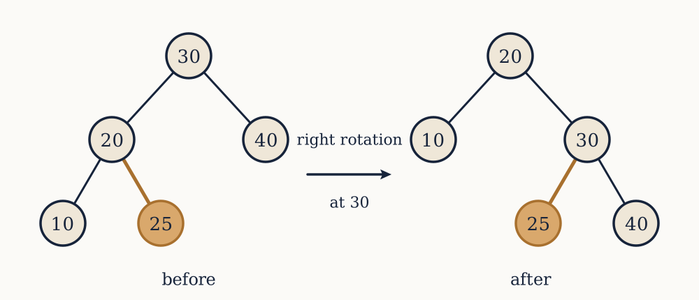
Example. A subtree has root 30 with left child 20 and right child 40, and 20 has children 10 and 25. Perform a right rotation at 30 and check the in-order sequence.

Before: in-order is 10, 20, 25, 30, 40. After the rotation, 20 is the subtree root, its left child is 10, its right child is 30, and 30 has left child 25 and right child 40. The subtree 25, which was right of 20, has become left of 30. In-order now reads 10, 20, 25, 30, 40, unchanged. The height of the subtree went from 2 to 2, but 10 rose from depth 2 to depth 1 and 40 fell from depth 1 to depth 2.

Now you. A subtree has root 50 with left child 40 and right child 70, and 70 has children 60 and 80. Perform a left rotation at 50.

Answer

70 becomes the subtree root. Its left child is 50, which keeps 40 on its left and takes 60 as its right child. Its right child is 80. In-order is 40, 50, 60, 70, 80 before and after. The subtree 60 was left of 70 and is now right of 50, and it sits between those two keys in value either way, which is why the move is legal.

The AVL rule

Rotations give the power to reshape. A balancing scheme is a rule saying when to use it. The first one, published by Georgy Adelson-Velsky and Evgenii Landis in 1962, is the strictest in common use.

An AVL tree requires that at every node, the heights of the two subtrees differ by at most 1. That difference is the node's balance factor, stored in the node as two bits.

Insert as in an ordinary binary search tree, then walk back up from the new leaf updating heights. The first node whose balance factor reaches 2 or $- 2$ is rebalanced, and there are four configurations, distinguished by which grandchild direction the new key went into.

If the insertion went into the left child's left subtree, one right rotation at the unbalanced node fixes it. Mirror-image for right-right. If it went into the left child's right subtree, a single rotation does not help: the middle subtree simply changes sides and the imbalance persists. That case needs a double rotation, a left rotation at the child followed by a right rotation at the node, which promotes the grandchild two levels. Mirror-image for right-left.

One rebalance, at most two rotations, restores the invariant for an insertion, and the walk back up is $O (h)$ , so insertion stays logarithmic. Deletion is slightly worse: fixing one node can shorten its subtree and unbalance its parent, so rebalancing may cascade all the way to the root, costing $O (\log n)$ rotations rather than a constant.

Example. Insert 50, 25, 75, 10, 30, 5 into an AVL tree. Where does the violation appear, and what fixes it?

The first five insertions are all legal: after them, 50 has children 25 and 75, and 25 has children 10 and 30. Inserting 5 puts it left of 10. Now 25 has a left subtree of height 1 and a right of height 0, a balance factor of 1, which is fine, but 50 has a left subtree of height 2 and a right of height 0, a balance factor of 2. The insertion went into 50's left child's left subtree, so this is the left-left case: one right rotation at 50. Afterwards 25 is the root, with left child 10 (holding 5) and right child 50 (holding 30 on the left and 75 on the right). Both of the root's subtrees now have height 1.

Now you. Insert 50, 25, 75, 10, 30, 27 instead.

Answer

27 goes left of 30. Node 50 again reaches balance factor 2, but the insertion went into its left child's right subtree, so this is the left-right case and one rotation is not enough. Left-rotate at 25 first, which lifts 30 into 25's place with 25 as its left child holding 10 and 27. Then right-rotate at 50. The result is 30 at the root, with left child 25 (children 10 and 27) and right child 50 (right child 75). In-order reads 10, 25, 27, 30, 50, 75, and the tree is balanced.

Why the bound is a Fibonacci argument

The invariant is local, and the height bound that follows from it is not obvious. Get at it by asking the opposite question: what is the fewest nodes an AVL tree of height $h$ can contain? A sparse tall tree is the worst case, so bounding sparseness bounds height.

Call that minimum $N (h)$ . Such a tree has a root, and to be as sparse as possible its two subtrees should be as sparse as possible while still legal: one of height $h - 1$ and, since the difference may be 1, the other of height $h - 2$ . So

N (h) = N (h - 1) + N (h - 2) + 1

with $N (0) = 1$ and $N (1) = 2$ . That is the Fibonacci recurrence with an offset, and indeed $N (h) = F (h + 3) - 1$ where $F$ is the usual Fibonacci sequence. The values run 1, 2, 4, 7, 12, 20, 33, 54, 88, 143.

Since $F (k)$ grows like $φ^{k} / \sqrt{5}$ with $φ = 1.618$ , $N (h)$ grows like $φ^{h}$ , so $h$ grows like $\log_{φ} n$ . Converting the base, $\log_{φ} n = \log_{2} n / \log_{2} φ = 1.4404 \log_{2} n$ , which gives the standard bound

h \leq 1.4405 \log_{2} (n + 2) - 0.3277

For a million keys that evaluates to 28.4, and running the recurrence exactly shows the true maximum height is 27, against 19 for a perfectly balanced tree. So the worst possible AVL tree is 44 per cent taller than the best possible tree, and that is a worst case on every input, not an average over random ones. Compare the unbalanced tree's worst case of 999,999.

Red-black trees and the cost of strictness

AVL's invariant is tight, which makes lookups fast and updates expensive: every insertion and deletion must maintain exact heights, and deletions can rotate all the way up.

Red-black trees, from Rudolf Bayer's 1972 symmetric binary B-trees as reformulated by Guibas and Sedgewick in 1978, relax it. Each node is coloured red or black, the root and the leaves are black, a red node's children are both black, and every root-to-leaf path contains the same number of black nodes. The last two rules together mean the longest path is at most twice the shortest, since the longest alternates red and black and the shortest is all black. The height bound is

h \leq 2 \log_{2} (n + 1)

which is 39.9 for a million keys against AVL's exact worst case of 27. Lookups therefore cost up to about 48 per cent more comparisons. In return, an insertion needs at most two rotations and a deletion at most three, both constants, with the rest of the repair done by recolouring, which is cheaper than pointer surgery.

That trade is why red-black trees are the ones actually shipped. C++'s std::map and std::set, Java's TreeMap and the Linux kernel's interval and process schedulers are all red-black. AVL survives where reads vastly outnumber writes. Two other schemes are worth knowing: treaps give each key a random priority and keep a heap order on priorities, achieving the random-tree behaviour of the previous lesson deliberately rather than by luck, and splay trees do not balance at all but rotate every accessed node to the root, giving $O (\log n)$ amortised cost and making recently used keys cheap.

Wide nodes

Every scheme so far assumed two children per node, and that assumption is worth questioning, because on real hardware the cost of a tree operation is not the comparison count but the number of memory locations touched.

Reading one byte from a spinning disk costs about 10 milliseconds and delivers a whole 4 KB page for the same price. Reading one byte from main memory costs about 100 nanoseconds and delivers a 64-byte cache line. In both cases the transfer is nearly free once the seek is paid, so the right structure fills the transfer unit with keys.

A B-tree, from Bayer and McCreight in 1972, does exactly that. Each node holds many keys in sorted order, say $b - 1$ of them, and has $b$ children, one for each gap between and beyond them. Searching a node means a binary search within it, which is free because the node is already in memory; descending means one more page read. All leaves sit at the same depth, and the tree grows by splitting a full node and pushing its middle key up into the parent, so it grows at the root rather than the leaves.

The arithmetic is the reason the structure exists. With a 16 KB page and 16 bytes per entry, $b = 1000$ . The root holds about 1000 keys, its 1000 children about $10^{6}$ , and their $10^{6}$ children about $10^{9}$ . So a billion keys sit three node reads from the root, and since the root and often the whole second level stay cached, most lookups cost one or two disk reads. A red-black tree over the same billion keys is up to 59 levels of pointer chasing, each one potentially its own seek.

Example. Compare the worst-case height of an AVL tree, a red-black tree and a B-tree with $b = 1000$ , all holding a billion keys.

$\log_{2} (10^{9}) = 29.9$ . AVL is bounded by $1.4405 \times 29.9 - 0.33 = 42.7$ , and running the Fibonacci recurrence gives an exact maximum of 41. Red-black is bounded by $2 \times 29.9 = 59.8$ , so 59. The B-tree needs $\log_{1000} (10^{9}) = 3$ levels. The binary trees are within a small constant of each other and the B-tree is an order of magnitude shallower, entirely because each of its nodes settles ten bits of the answer instead of one.

Now you. How deep is that B-tree for a trillion keys, and how tall could the AVL tree get?

Answer

$\log_{1000} (10^{12}) = 4$ levels for the B-tree. For AVL, $\log_{2} (10^{12}) = 39.86$ , so the bound is $1.4405 \times 39.86 - 0.33 = 57.1$ . A thousand times more keys cost the B-tree one extra read and the AVL tree fourteen extra levels. This is why every relational database index, and every filesystem from NTFS to ext4 to APFS, is a B-tree or a close relative rather than a binary tree.

What is now available

Between them, the last three lessons deliver an ordered dictionary: insert, delete, look up, find the minimum, find the successor, and list a range, all in guaranteed $O (\log n)$ with an in-order walk in $Θ (n)$ . A hash table is faster for exact lookup and cannot do the rest. That is the whole trade, and it is enough to choose between them for almost any real problem.

It is also more than many problems need. A great many tasks never ask for a general lookup at all: they repeatedly ask for the smallest remaining item, or the largest, and nothing else. A scheduler wants the next job to run, a simulation wants the next event, a compressor wants the two least frequent symbols. Maintaining a full ordering to answer that one question is paying for an invariant that is never queried.

The next lesson keeps a much weaker invariant, only that each node is smaller than its children, which is loose enough to be maintained in a plain array with no pointers at all, and strong enough to hand over the minimum in constant time.