Hash tables

A sorted array answers a lookup in about $\log_{2} n$ comparisons, twenty of them for a million keys, and the previous lesson showed that no comparison-based method does better.

Twenty is not many. But a comparison sort is bound by that floor only because it insists on comparing, and the non-comparison sorts escaped it by using a key as an address instead. The same escape is available to searching, and it is worth far more there: it turns lookup from logarithmic into constant, independent of how many keys the structure holds.

Direct addressing, and why it does not scale

Start with the extreme case. If keys are integers from 0 to $k - 1$ and each is used at most once, allocate an array of $k$ slots and store the record for key $x$ at index $x$ . Lookup, insertion and deletion are one array access each, and there is nothing to analyse.

This is a direct-address table, and it is genuinely the right structure sometimes: a lookup by day of the year, by byte value, by HTTP status code. Its cost is $Θ (k)$ memory regardless of how many keys are actually present.

That is what kills it in general. To store ten thousand customer records keyed by a nine-digit identifier, direct addressing wants a billion slots to hold ten thousand entries, a millionth of them occupied. The keys are drawn from an enormous universe $U$ but only a tiny subset is ever present, and the table pays for the universe.

The fix is to compress the universe. Pick a table size $m$ close to the number of keys expected, and a hash function $h$ mapping $U$ into ${0, 1, \dots, m - 1}$ . Store the record for key $x$ at index $h (x)$ . Memory is now $Θ (m)$ rather than $Θ (| U |)$ , and computing $h (x)$ is a fixed amount of arithmetic that does not grow with $n$ .

The commonest hash for integer keys is the division method, $h (x) = x mod m$ , with $m$ prime and not close to a power of two, since $m = 2^{p}$ makes $h$ depend on the low $p$ bits alone and throws away the rest of the key. For strings, the standard trick is to treat the characters as digits in some base: Java's String.hashCode computes $\sum s_{i} \cdot 31^{n - 1 - i}$ over a 32-bit integer, and 31 is chosen because it is prime, odd, and $31 x$ is computable as a shift and a subtract.

Collisions are not a risk, they are arithmetic

Since $| U | > m$ , there must be two distinct keys with the same hash value. This is the pigeonhole principle and it admits no cleverness: no hash function whatever, however well designed, avoids collisions on a universe larger than its range.

Worse, collisions arrive far earlier than intuition suggests. Insert $n$ random keys into $m$ slots. The probability that all $n$ land in different slots is the product $\frac{m}{m} \cdot \frac{m - 1}{m} \dots \frac{m - n + 1}{m}$ , which falls below one half at roughly $n = 1.177 \sqrt{m}$ . This is the birthday problem: with $m = 365$ the answer is 23 people.

Example. A hash table has a million slots. How many random keys can be inserted before a collision is more likely than not?

Multiplying out $\prod_{i = 0}^{n - 1} (1 - i / 10^{6})$ until it drops below 0.5 gives $n = 1178$ . The approximation $1.177 \sqrt{10^{6}} = 1177$ agrees. So a table with a million slots and just over a thousand keys, occupancy of about one part in a thousand, is already at even odds of a collision.

Now you. How many keys is that for a table of a thousand slots?

Answer

$1.177 \sqrt{1000} = 37.2$ , and the exact product first falls below one half at $n = 38$ . Collision handling is not an edge case to bolt on later; it is most of the design of a hash table.

Chaining

The first resolution scheme is to stop insisting that a slot holds one record. In separate chaining, slot $i$ holds a linked list of every record whose key hashes to $i$ . Insertion prepends to the list in constant time. Lookup hashes, then walks that one list.

The analysis needs a name for how full the table is. The load factor is $α = n / m$ , the average number of keys per slot, and with chaining it may exceed 1.

Assume simple uniform hashing: each key is equally likely to hash to any slot, independently of the others. Then an unsuccessful search examines a list of expected length $α$ , so its expected cost is $1 + α$ counting the hash itself. A successful search finds the target part-way along its list, and averaging over the keys gives $1 + α / 2$ roughly. Both are constant when $α$ is held constant, and that is the whole result: hash table operations are $Θ (1)$ expected, provided the load factor is bounded.

The worst case is untouched by this. If every key hashes to the same slot, the table is one linked list and lookup is $Θ (n)$ . Expected constant time is a statement about the distribution of keys, not a guarantee about any particular set of them.

Open addressing

Chaining spends a pointer per record and scatters the records across the heap, which is expensive on hardware that rewards locality. Open addressing stores every record in the table itself and, when a slot is taken, probes a sequence of further slots until it finds a free one.

Linear probing is the simplest: try $h (x)$ , then $h (x) + 1$ , then $h (x) + 2$ , wrapping around. It was used by Gene Amdahl, Elaine McGraw and Arthur Samuel in 1954 in the assembler for the IBM 701, and Knuth's analysis of it in 1963 is the paper he credits with turning him towards the analysis of algorithms.

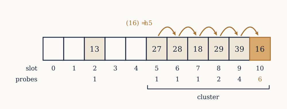
Example. Insert 27, 18, 29, 28, 39, 13, 16 into a table of 11 slots with $h (x) = x mod 11$ and linear probing, counting probes.

The hashes are 5, 7, 7, 6, 6, 2, 5. Key 27 takes slot 5 in one probe, 18 takes 7 in one. Key 29 hashes to 7, which is taken, so it lands at 8 in two probes. Key 28 takes 6 in one. Key 39 hashes to 6 and finds 6, 7 and 8 occupied, landing at 9 in four probes. Key 13 takes 2 in one. Key 16 hashes to 5 and walks 5, 6, 7, 8, 9 before reaching 10, six probes. Total 16 probes for seven insertions, an average of 2.29, at a load factor of $7 / 11 = 0.64$ .

Now you. Insert 45, 31, 12, 23, 56, 19, 7 into a table of 13 slots with $h (x) = x mod 13$ .

Answer

Hashes 6, 5, 12, 10, 4, 6, 7. The first five keys all find their home slot free, one probe each. Key 19 hashes to 6, taken by 45, so it lands at 7 in two probes. Key 7 hashes to 7, now taken by 19, so it lands at 8 in two probes. Total 9 probes, an average of 1.29 at a load factor of $7 / 13 = 0.54$ . The same seven keys in a table one fifth larger cost 44 per cent fewer probes, which is what the next section quantifies.

Linear probing has a specific pathology visible in that first example: keys 5 to 10 formed a single occupied block, and any key hashing anywhere into it walks to the end. This is primary clustering. A long run grows faster than a short one, because it presents a wider target, so runs snowball. Quadratic probing, stepping by $1, 4, 9, \dots$ , and double hashing, stepping by a second hash of the key, break the clusters up at the cost of losing the sequential memory access that made linear probing fast in the first place.

Deletion under open addressing needs care. Emptying a slot outright breaks every probe sequence that ran through it, so a deleted slot is marked with a tombstone that probing walks past but insertion may reuse. Tombstones accumulate and are cleared by rebuilding.

What the load factor buys

The probe counts are all functions of $α$ alone, and never of $n$ . Under uniform hashing, an unsuccessful search costs about $1 / (1 - α)$ probes and a successful one about $(1 / α) \ln (1 / (1 - α))$ . Linear probing, with its clustering, is worse: Knuth's results give about $\frac{12}{(} 1 + 1 / (1 - α))$ probes for a successful search and $\frac{12}{(} 1 + 1 / (1 - α)^{2})$ for an unsuccessful one.

Those formulas explode near $α = 1$ , and the numbers are worth seeing. At $α = 0.5$ , linear probing takes 1.5 probes for a hit and 2.5 for a miss. At $α = 0.75$ , 2.5 and 8.5. At $α = 0.9$ , 5.5 and 50.5. At $α = 0.95$ , 10.5 and 200.5. The cost is flat until the table is about three quarters full and then goes off a cliff.

Example. A linear-probing table of 1024 slots holds 768 keys. What does a search cost, and what does doubling the table to 2048 slots do?

The load factor is $768 / 1024 = 0.75$ , so a hit costs $\frac{12}{(} 1 + 4) = 2.5$ probes and a miss $\frac{12}{(} 1 + 16) = 8.5$ . Doubling gives $α = 0.375$ , so a hit costs $\frac{12}{(} 1 + 1.6) = 1.30$ and a miss $\frac{12}{(} 1 + 2.56) = 1.78$ . Doubling the memory cut the miss cost by a factor of 4.8.

Now you. The same table has 4096 slots and 3686 keys. What do a hit and a miss cost, and what would chaining cost instead?

Answer

$α = 3686 / 4096 = 0.90$ . Linear probing gives $\frac{12}{(} 1 + 10) = 5.5$ probes for a hit and $\frac{12}{(} 1 + 100) = 50.5$ for a miss. Chaining at the same load factor costs $1 + α / 2 = 1.45$ for a hit and $1 + α = 1.9$ for a miss, because a chained table degrades linearly in $α$ rather than exploding. This is why open addressing is resized aggressively and chaining is not.

So the table must be kept below some threshold, which means resizing when it fills. Allocate a table of double the size and reinsert every key, since a key's slot depends on $m$ and no old position survives. That rehash costs $Θ (n)$ , and it is exactly the growable-array argument from the third lesson: doubling makes the total cost of $n$ insertions $Θ (n)$ , so the amortised cost per insertion stays constant. The threshold is a tuning decision, and real implementations differ: Java's HashMap resizes at 0.75, Python's dictionary at about 0.66, and Google's Swiss tables at around 0.875 because their probing is done sixteen slots at a time with vector instructions.

When the keys are chosen by an attacker

Every result above assumed the keys were not adversarial. Drop that assumption and expected constant time disappears completely.

If an attacker knows the hash function, they can compute a set of keys that all collide, and feed them in. A table with $n$ colliding keys degrades to a linked list, so $n$ insertions cost $Θ (n^{2})$ . Crosby and Wallach demonstrated this in 2003 against the Bro intrusion detection system and against Perl. At the 2011 Chaos Communication Congress, Klink and Wälde showed the same attack against the form-parsing code of PHP, Java, Python, Ruby and ASP.NET: a single HTTP POST of a few hundred kilobytes of colliding parameter names could occupy a server core for minutes.

The repair is a randomised hash: a family of functions with a per-process random seed chosen at startup, so the attacker cannot know which function is in use. Python enabled seed randomisation by default in version 3.3 in 2012, and SipHash, published by Aumasson and Bernstein the same year, is a keyed hash fast enough for short strings and designed for this exact role. Java took a different route in version 8: a HashMap bucket whose chain exceeds eight entries is converted to a balanced tree, so the worst case becomes $Θ (\log n)$ rather than $Θ (n)$ . That tree is the subject of the next two lessons.

What was traded away

A hash table gives expected constant-time insert, delete and lookup by exact key, at the price of the worst case, some memory to hold the load factor down, and a rehash whenever the table doubles. For lookup by exact key it is very hard to beat.

The price is order. A hash function's whole job is to scatter keys that were near each other in value, so the table has no notion of sequence at all. It cannot report the smallest key, or the next key after a given one, or every key between two bounds, or the keys in order, without inspecting all $m$ slots and sorting them. In exchange for constant lookup it has destroyed every question except "is this exact key here?".

Many real questions are the other kind: the ten most recent entries, everything between two timestamps, the next available identifier. The next lesson builds a structure that keeps the halving behaviour of binary search while allowing insertion and deletion, which means keeping the keys ordered as they arrive, and it costs a factor of $\log n$ against the hash table to do it.